1 Introduction

This website is a supplement to the paper The impact of dyads and extended networks on political talk: A factorial survey experiment in the Netherlands It contains the link to the publicly available data set we used NELLS and all the necessary R code to replicate our reported results and tables.

Hofstra, B., Jeroense, T., Tolsma, J. (2026). The impact of dyads and extended networks on political talk: A factorial survey experiment in the Netherlands. Social Networks, 85, 66-67 pdf doi

1.1 Contact

Questions can be addressed to Bas Hofstra

1.2 general custom functions

fpackage.check: Check if packages are installed (and install if not) in R
fsave: Function to save data with time stamp in correct directory
fload: Function to load R-objects under new names
fshowdf: Print objects (tibble / data.frame) nicely on screen in .Rmd
ftheme: pretty ggplot2 theme

fpackage.check <- function(packages) {
    lapply(packages, FUN = function(x) {
        if (!require(x, character.only = TRUE)) {
            install.packages(x, dependencies = TRUE)
            library(x, character.only = TRUE)
        }
    })
}

fsave <- function(x, location = "./data/processed/") {
    if (location == "./data/processed/") {
        ifelse(!dir.exists("data"), dir.create("data"), FALSE)
        ifelse(!dir.exists("data/processed"), dir.create("data/processed"), FALSE)
    }

    object = deparse(substitute(x))
    datename <- substr(gsub("[:-]", "", Sys.time()), 1, 8)
    totalname <- paste(location, object, "_", datename, ".rda", sep = "")
    assign(eval(object), x, envir = .GlobalEnv)
    print(paste("SAVED: ", totalname, sep = ""))
    save(list = object, file = totalname)
}

fload <- function(fileName) {
    load(fileName)
    get(ls()[ls() != "fileName"])
}


fshowdf <- function(x, caption = NULL, ...) {
    knitr::kable(x, digits = 2, "html", caption = caption, ...) %>%
        kableExtra::kable_styling(bootstrap_options = c("striped", "hover")) %>%
        kableExtra::scroll_box(width = "100%", height = "300px")
}

ftheme <- function() {
    # download font at https://fonts.google.com/specimen/Jost/
    theme_minimal(base_family = "Jost") + theme(panel.grid.minor = element_blank(), plot.title = element_text(family = "Jost",
        face = "bold"), axis.title = element_text(family = "Jost Medium"), axis.title.x = element_text(hjust = 0),
        axis.title.y = element_text(hjust = 1), strip.text = element_text(family = "Jost", face = "bold",
            size = rel(0.75), hjust = 0), strip.background = element_rect(fill = "grey90", color = NA),
        legend.position = "bottom")
}

1.3 necessary packages

To further ease replication purposes we use groundhog.

packages <- c("tidyverse", "lme4", "psych", "ordinal", "ggplot2", "officer", "flextable", "Hmisc", "jtools",
    "parallel")
fpackage.check(packages)

1.4 session info

sessionInfo()

#> R version 4.4.2 (2024-10-31 ucrt)
#> Platform: x86_64-w64-mingw32/x64
#> Running under: Windows 11 x64 (build 26100)
#> 
#> Matrix products: default
#> 
#> 
#> locale:
#> [1] LC_COLLATE=English_United Kingdom.utf8  LC_CTYPE=English_United Kingdom.utf8   
#> [3] LC_MONETARY=English_United Kingdom.utf8 LC_NUMERIC=C                           
#> [5] LC_TIME=English_United Kingdom.utf8    
#> 
#> time zone: Europe/Amsterdam
#> tzcode source: internal
#> 
#> attached base packages:
#> [1] stats     graphics  grDevices utils     datasets  methods   base     
#> 
#> other attached packages:
#>  [1] jtools_2.3.0        Hmisc_5.1-3         flextable_0.9.6     officer_0.6.6      
#>  [5] ordinal_2023.12-4.1 psych_2.4.6.26      lme4_1.1-35.5       Matrix_1.7-0       
#>  [9] lubridate_1.9.3     forcats_1.0.0       stringr_1.5.1       dplyr_1.1.4        
#> [13] purrr_1.0.2         readr_2.1.5         tidyr_1.3.1         tibble_3.2.1       
#> [17] ggplot2_3.5.1       tidyverse_2.0.0     groundhog_3.2.1     knitr_1.48         
#> 
#> loaded via a namespace (and not attached):
#>  [1] mnormt_2.1.1            gridExtra_2.3           formatR_1.14            rlang_1.1.4            
#>  [5] magrittr_2.0.3          furrr_0.3.1             compiler_4.4.2          systemfonts_1.1.0      
#>  [9] vctrs_0.6.5             pkgconfig_2.0.3         fastmap_1.2.0           backports_1.5.0        
#> [13] pander_0.6.5            utf8_1.2.4              rmarkdown_2.28          tzdb_0.4.0             
#> [17] nloptr_2.1.1            ragg_1.3.3              xfun_0.48               cachem_1.1.0           
#> [21] jsonlite_1.8.9          uuid_1.2-1              broom_1.0.7             parallel_4.4.2         
#> [25] cluster_2.1.6           R6_2.5.1                bslib_0.8.0             stringi_1.8.4          
#> [29] parallelly_1.38.0       boot_1.3-31             extrafontdb_1.0         rpart_4.1.23           
#> [33] jquerylib_0.1.4         numDeriv_2016.8-1.1     Rcpp_1.0.13             assertthat_0.2.1       
#> [37] klippy_0.0.0.9500       base64enc_0.1-3         extrafont_0.19          splines_4.4.2          
#> [41] nnet_7.3-19             timechange_0.3.0        tidyselect_1.2.1        rstudioapi_0.16.0      
#> [45] yaml_2.3.10             codetools_0.2-20        listenv_0.9.1           lattice_0.22-6         
#> [49] withr_3.0.1             askpass_1.2.1           evaluate_1.0.0          foreign_0.8-87         
#> [53] future_1.34.0           zip_2.3.1               xml2_1.3.6              pillar_1.9.0           
#> [57] checkmate_2.3.2         generics_0.1.3          hms_1.1.3               munsell_0.5.1          
#> [61] scales_1.3.0            minqa_1.2.8             globals_0.16.3          glue_1.8.0             
#> [65] gdtools_0.4.0           tools_4.4.2             data.table_1.16.0       rgl_1.3.14             
#> [69] grid_4.4.2              Rttf2pt1_1.3.12         colorspace_2.1-1        nlme_3.1-166           
#> [73] htmlTable_2.4.3         Formula_1.2-5           cli_3.6.3               textshaping_0.4.0      
#> [77] fontBitstreamVera_0.1.1 fansi_1.0.6             gtable_0.3.5            broom.mixed_0.2.9.5    
#> [81] sass_0.4.9              digest_0.6.37           fontquiver_0.2.1        ucminf_1.2.2           
#> [85] htmlwidgets_1.6.4       htmltools_0.5.8.1       lifecycle_1.0.4         fontLiberation_0.1.0   
#> [89] openssl_2.2.2           MASS_7.3-61

2 NELLS

We use the third wave of the NEtherlands Longitudinal Lifecourse Study (Jeroense et al. 2023). This dataset is publically available at DANS Data Station Social Sciences and Humanities, see https://doi.org/10.17026/DANS-XYK-M56B. Please make sure to download the dataset with the variables that were originally under embargo included.

# df <- fload('Data/2023-04-06_nells-cleaned-22-V1.0.Rdata')
df_dans <- fload("Data/nells-22_V1.1.Rdata")
df <- df_dans

2.1 gender and ethnic background

df$female <- as.numeric(df$B02 == 2)  #gender

# etnicity, no missings
df$egoNL <- as.numeric(df$B05 == 1 & df$B06 == 1 & df$B07 == 1)
df$egoM <- as.numeric(df$B05 == 2 | df$B06 == 2 | df$B07 == 2)
df$egoT <- as.numeric(df$B05 == 3 | df$B06 == 3 | df$B07 == 3)
df$egoM <- ifelse(df$B06 == 2, 1, df$egoM)  #mother dominant
df$egoT <- ifelse(df$B06 == 3, 1, df$egoT)  #mother dominant
df$egoO <- as.numeric(df$egoNL != 1 & df$egoM != 1 & df$egoT != 1)  #other, need to filter
# generation
df$ego_gen1 <- as.numeric(df$B05 == 2 | df$B05 == 3)

# table(df$egoM, useNA = 'always') table(df$egoT, useNA = 'always') table(df$egoO, useNA =
# 'always') #need to filter

2.2 age and education

# age table(is.na(df$cage))

# education
df$educL <- as.numeric(df$C05 < 5 | df$C05 == 13)  # lower than Havo
df$educM <- as.numeric((df$C05 > 4 & df$C05 < 9) | df$C05 == 14)  # have, vwo, mbo
df$educH <- as.numeric((df$C05 > 8 & df$C05 < 13) | df$C05 == 15)  # hbo, wo
df$educ_current <- as.numeric(df$C03 == 1)  # currently full-time in educ

2.3 additional potential controls

# political opinions H12d. De overheid moet de inkomensverschillen in Nederland kleiner maken H12e.
# De topinkomens in het bedrijfsleven zijn te hoog H12f. De overheid moet de sociale uitkeringen
# verhogen attributes(df$H12e)

df$ego_opinion1 <- df$H12e
df$ego_opinion1b <- rowMeans(cbind(df$H12d, df$H12e, df$H12f), na.rm = T)
# table(df$ego_opinion1, useNA = 'always')

# H12a. Als een land spanningen wil verminderen moet de immigratie stoppen
df$ego_opinion2 <- df$H12a
# attributes(df$H12a) reverse coding
df$ego_opinion2 <- 6 - df$ego_opinion2

# H13d. Het klimaat verbeteren moet prioriteit hebben, zelfs als dit de economische groei vertraagt
df$ego_opinion3 <- df$H13d
# table(df$ego_opinion3, useNA = 'always') attributes(df$H13d)

df %>%
    select(c(ego_opinion1, ego_opinion2, ego_opinion3, ego_opinion1b, H12d, H12e, H12f)) %>%
    as.matrix() %>%
    Hmisc::rcorr()

# feeling thermometers
df$thermoD <- df$H19i
df$thermoM <- df$H19j
df$thermoT <- df$H19k

# H06. Political interest
df$polint <- df$H06
# table(df$H06, useNA = 'always') attributes(df$H06)

# district variables: gender and ethnic diversity
df <- df %>%
    mutate(cdistrict2020_a_nl = cdistrict2020_a_inw - cdistrict2020_a_w_all - cdistrict2020_a_w_all,
        district_EI_ethnic = case_when(egoNL == 1 ~ (cdistrict2020_a_nl - (cdistrict2020_a_inw - cdistrict2020_a_nl))/cdistrict2020_a_inw,
            egoM == 1 ~ (cdistrict2020_a_marok - (cdistrict2020_a_inw - cdistrict2020_a_marok))/cdistrict2020_a_inw,
            egoT == 1 ~ (cdistrict2020_a_tur - (cdistrict2020_a_inw - cdistrict2020_a_tur))/cdistrict2020_a_inw,
            .default = NA), district_EI_gender = case_when(female == 1 ~ (cdistrict2020_a_vrouw - cdistrict2020_a_man)/(cdistrict2020_a_vrouw +
            cdistrict2020_a_man), female == 0 ~ (cdistrict2020_a_man - cdistrict2020_a_vrouw)/(cdistrict2020_a_vrouw +
            cdistrict2020_a_man))) %>%
    mutate(district_EI_ethnic = ifelse(district_EI_ethnic > 1 | district_EI_ethnic < -1, NA, district_EI_ethnic),
        district_EI_gender = ifelse(district_EI_gender > 1 | district_EI_gender < -1, NA, district_EI_gender))

# Core Discussion Network (size of non-kin network, gender/ethnic EI )
df <- df %>%
    mutate(across(I02a:I05e, ~replace_na(.x, -1))  #replace NA's with -1
) %>%
    mutate(cdn_tot = 5 - rowSums(cbind(is.na(df$calter_id1), is.na(df$calter_id2), is.na(df$calter_id3),
        is.na(df$calter_id4), is.na(df$calter_id5)))) %>%
    rowwise() %>%
    # to be able to count values across variables for each row
mutate(nka = !(I02a < 4 & I02a > 1), nkb = !(I02b < 4 & I02b > 1), nkc = !(I02c < 4 & I02c > 1), nkd = !(I02d <
    4 & I02d > 1), nke = !(I02e < 4 & I02e > 1), cdn_tot_nk = cdn_tot - sum(c(I02a < 4 & I02a > 1, I02b <
    4 & I02b > 1, I02c < 4 & I02c > 1, I02d < 4 & I02d > 1, I02e < 4 & I02e > 1)), cdn_NL = sum(c(nka &
    I04a == 1, nkb & I04b == 1, nkc & I04c == 1, nkd & I04d == 1, nke & I04e == 1)), cdn_M = sum(c(nka &
    I04a == 2, nkb & I04b == 2, nkc & I04c == 2, nkd & I04d == 2, nke & I04e == 2)), cdn_T = sum(c(nka &
    I04a == 3, nkb & I04b == 3, nkc & I04c == 3, nkd & I04d == 3, nke & I04e == 3)), cdn_O = sum(c(nka &
    I04a == 4, nkb & I04b == 4, nkc & I04c == 4, nkd & I04d == 4, nke & I04e == 4)), cdn_men = sum(c(nka &
    I03a == 1, nkb & I03b == 1, nkc & I03c == 1, nkd & I03d == 1, nke & I03e == 1)), cdn_women = sum(c(nka &
    I03a == 2, nkb & I03b == 2, nkc & I03c == 2, nkd & I03d == 2, nke & I03e == 2))) %>%
    ungroup() %>%
    # higher EI scores indicate more intragroup ties than intergroup ties. range -1 to 1, note only
    # relvant if size>0
mutate(cdn_EI_ethnic = case_when(egoNL == 1 ~ (cdn_NL - (cdn_tot_nk - cdn_NL))/cdn_tot_nk, egoM == 1 ~
    (cdn_M - (cdn_tot_nk - cdn_M))/cdn_tot_nk, egoT == 1 ~ (cdn_T - (cdn_tot_nk - cdn_T))/cdn_tot_nk,
    .default = NA), cdn_EI_gender = case_when(female == 1 ~ (cdn_women - (cdn_tot_nk - cdn_women))/cdn_tot_nk,
    female == 0 ~ (cdn_men - (cdn_tot_nk - cdn_men))/cdn_tot_nk, .default = NA)) %>%
    mutate(across(c(cdn_tot:cdn_EI_gender), ~ifelse(is.na(H19o) & is.na(J01a), NA, .))) %>%
    # if respondents did not answer questions, replace values with NA
mutate(cdn_EI_ethnic = ifelse(cdn_EI_ethnic > 1 | cdn_EI_ethnic < -1, NA, cdn_EI_ethnic), cdn_EI_gender = ifelse(cdn_EI_gender >
    1 | cdn_EI_gender < -1, NA, cdn_EI_gender))
# few data discrepancies table(df$cdn_EI_ethnic)

2.4 NSUM

For construction see here.

nsum <- fload("./Data/nsum_outcomes/nsum_size_diversity.rda")

2.4.1 diversity measures

Higher scores more diversity.

nsum$hhi_ethnic <- 1 - nsum$hhi_ethnic
nsum$hhi_gender <- 1 - nsum$hhi_gender
nsum$hhi_educ <- 1 - nsum$hhi_educ

df <- df %>%
    left_join(y = nsum)

# calculate the EI scores
df <- df %>%
    mutate(nsum_EI_ethnic = case_when(egoNL == 1 ~ (nsum_dut - (nsum_mor + nsum_tur))/(nsum_dut + nsum_mor +
        nsum_tur), egoM == 1 ~ (nsum_mor - (nsum_dut + nsum_tur))/(nsum_dut + nsum_mor + nsum_tur), egoT ==
        1 ~ (nsum_tur - (nsum_dut + nsum_mor))/(nsum_dut + nsum_mor + nsum_tur), .default = NA), nsum_EI_gender = case_when(female ==
        1 ~ (nsum_women - (nsum_men))/(nsum_women + nsum_men), female == 0 ~ (nsum_men - (nsum_women))/(nsum_women +
        nsum_men), .default = NA)) %>%
    mutate(nsum_EI_ethnic = ifelse(nsum_EI_ethnic > 1 | nsum_EI_ethnic < -1, NA, nsum_EI_ethnic), nsum_EI_gender = ifelse(nsum_EI_gender >
        1 | nsum_EI_gender < -1, NA, nsum_EI_gender))

2.5 Sample selection and missings

As described in our manuscript, NELLS applied a split ballot design. The NSUM items were only included in split ballot 2.

table(df$csplitballot, useNA = "always")
df_sb1 <- df[df$csplitballot == 1, ]  #1503
df_sb2 <- df[df$csplitballot == 2, ]  #1514

#> 
#>    1    2 <NA> 
#> 1503 1514    0

3 Table 1

To summarize the dimension of the survey experiment we report Table 1 in our manuscript.

Table 1. Dimensions of Survey experiment 'Political Talk'
Gender	Ethnic background	Relationship	Policy measure	Political distance
1. Man	1. Dutch	1. a colleague	1. introduce higher taxes for people with top incomes	1. thinks substantively more negative about this proposal than you
2. Woman	2. Moroccan	2. a good friend	2. allow less refugees access to the Netherlands	2. thinks substantively more positive about this proposal than you
	3. Turkish	3. an acquaintance	3. reduce subsidies for sustainability policies (for example electric cars, solar panels and heat pumps)	3. thinks about the same about this proposal than you
		4. family (in-laws)
		5. someone you just met

4 Table 2

Descriptives dependent variable.

We present descriptive for total sample, and per ethnic group. We do this for weighted sample and unweighted. For the total sample we weigh to (representative) Dutch population. For the ethnic group samples we weigh to (representative) ethnic group populations. See the codebook of NELLS for more details.

Our main conclusion is that distributions do not change substantially for weighted and unweighted samples. We therefore continue our analysis on an unweighted sample.

# from wide to long (we have two observation per resondent)
df1 <- df
df2 <- df
df1$index <- 1
df2$index <- 2
df_tot <- rbind(df1, df2)
df_tot$Y <- ifelse(df_tot$index == 1, df_tot$L1, df_tot$L2)
summary(df_tot$Y)

#>    Min. 1st Qu.  Median    Mean 3rd Qu.    Max.    NA's 
#>   1.000   3.000   4.000   3.864   5.000   5.000     931

4.1 number of respondents for total sample

df_sel <- df[!is.na(df$L1) & !is.na(df$L2), ]
# total
nrow(df_sel)
# etnicity
table(df_sel$egoNL, useNA = "always")
table(df_sel$egoM, useNA = "always")
table(df_sel$egoT, useNA = "always")
# gender
table(df_sel$female, useNA = "always")

#> [1] 2545
#> 
#>    0    1 <NA> 
#> 1064 1481    0 
#> 
#>    0    1 <NA> 
#> 2139  406    0 
#> 
#>    0    1 <NA> 
#> 1910  635    0 
#> 
#>    0    1 <NA> 
#> 1193 1352    0

# present result for a weighted sample, and for an unweighted sample
myw <- wtd.mean(df_tot$Y, weights = df_tot$cweight2, normwt = TRUE)
my <- wtd.mean(df_tot$Y)

propyw <- round(prop.table(wtd.table(df_tot$Y, weights = df_tot$cweight2, normwt = TRUE)$sum.of.weights),
    3)
propy <- round(prop.table(wtd.table(df_tot$Y)$sum.of.weights), 3)

Nobsw <- round(sum(wtd.table(df_tot$Y, weights = df_tot$cweight2, normwt = TRUE)$sum.of.weights), 3)
Nobs <- round(sum(wtd.table(df_tot$Y)$sum.of.weights), 3)

resw <- c(propyw, myw, Nobsw)
res <- c(propy, my, Nobs)

# Per ethnic group nl
myw <- wtd.mean(df_tot$Y[df_tot$egoNL == 1], weights = df_tot$cweight1[df_tot$egoNL == 1], normwt = TRUE)
my <- wtd.mean(df_tot$Y[df_tot$egoNL == 1])

propyw <- round(prop.table(wtd.table(df_tot$Y[df_tot$egoNL == 1], weights = df_tot$cweight1[df_tot$egoNL ==
    1], normwt = TRUE)$sum.of.weights), 3)
propy <- round(prop.table(wtd.table(df_tot$Y[df_tot$egoNL == 1])$sum.of.weights), 3)

Nobsw <- round(sum(wtd.table(df_tot$Y[df_tot$egoNL == 1], weights = df_tot$cweight1[df_tot$egoNL == 1],
    normwt = TRUE)$sum.of.weights), 3)
Nobs <- round(sum(wtd.table(df_tot$Y[df_tot$egoNL == 1])$sum.of.weights), 3)

reswN <- c(propyw, myw, Nobsw)
resN <- c(propy, my, Nobs)


# m
myw <- wtd.mean(df_tot$Y[df_tot$egoM == 1], weights = df_tot$cweight1[df_tot$egoM == 1], normwt = TRUE)
my <- wtd.mean(df_tot$Y[df_tot$egoM == 1])

propyw <- round(prop.table(wtd.table(df_tot$Y[df_tot$egoM == 1], weights = df_tot$cweight1[df_tot$egoM ==
    1], normwt = TRUE)$sum.of.weights), 3)
propy <- round(prop.table(wtd.table(df_tot$Y[df_tot$egoM == 1])$sum.of.weights), 3)

Nobsw <- round(sum(wtd.table(df_tot$Y[df_tot$egoM == 1], weights = df_tot$cweight1[df_tot$egoM == 1],
    normwt = TRUE)$sum.of.weights), 3)
Nobs <- round(sum(wtd.table(df_tot$Y[df_tot$egoM == 1])$sum.of.weights), 3)

reswM <- c(propyw, myw, Nobsw)
resM <- c(propy, my, Nobs)

# t
myw <- wtd.mean(df_tot$Y[df_tot$egoT == 1], weights = df_tot$cweight1[df_tot$egoT == 1], normwt = TRUE)
my <- wtd.mean(df_tot$Y[df_tot$egoT == 1])

propyw <- round(prop.table(wtd.table(df_tot$Y[df_tot$egoT == 1], weights = df_tot$cweight1[df_tot$egoT ==
    1], normwt = TRUE)$sum.of.weights), 3)
propy <- round(prop.table(wtd.table(df_tot$Y[df_tot$egoT == 1])$sum.of.weights), 3)

Nobsw <- round(sum(wtd.table(df_tot$Y[df_tot$egoT == 1], weights = df_tot$cweight1[df_tot$egoT == 1],
    normwt = TRUE)$sum.of.weights), 0)
Nobs <- round(sum(wtd.table(df_tot$Y[df_tot$egoT == 1])$sum.of.weights), 0)

reswT <- c(propyw, myw, Nobsw)
resT <- c(propy, my, Nobs)

# men
myw <- wtd.mean(df_tot$Y[df_tot$female == 0], weights = df_tot$cweight1[df_tot$female == 0], normwt = TRUE)
my <- wtd.mean(df_tot$Y[df_tot$female == 0])

propyw <- round(prop.table(wtd.table(df_tot$Y[df_tot$female == 0], weights = df_tot$cweight1[df_tot$female ==
    0], normwt = TRUE)$sum.of.weights), 3)
propy <- round(prop.table(wtd.table(df_tot$Y[df_tot$female == 0])$sum.of.weights), 3)

Nobsw <- round(sum(wtd.table(df_tot$Y[df_tot$female == 0], weights = df_tot$cweight1[df_tot$female ==
    0], normwt = TRUE)$sum.of.weights), 0)
Nobs <- round(sum(wtd.table(df_tot$Y[df_tot$female == 0])$sum.of.weights), 0)

reswMen <- c(propyw, myw, Nobsw)
resMen <- c(propy, my, Nobs)

# women
myw <- wtd.mean(df_tot$Y[df_tot$female == 1], weights = df_tot$cweight1[df_tot$female == 1], normwt = TRUE)
my <- wtd.mean(df_tot$Y[df_tot$female == 1])

propyw <- round(prop.table(wtd.table(df_tot$Y[df_tot$female == 1], weights = df_tot$cweight1[df_tot$female ==
    1], normwt = TRUE)$sum.of.weights), 3)
propy <- round(prop.table(wtd.table(df_tot$Y[df_tot$female == 1])$sum.of.weights), 3)

Nobsw <- round(sum(wtd.table(df_tot$Y[df_tot$female == 1], weights = df_tot$cweight1[df_tot$female ==
    1], normwt = TRUE)$sum.of.weights), 0)
Nobs <- round(sum(wtd.table(df_tot$Y[df_tot$female == 1])$sum.of.weights), 0)

reswWomen <- c(propyw, myw, Nobsw)
resWomen <- c(propy, my, Nobs)

res2 <- as_tibble(cbind(res, resw, resWomen, reswWomen, resMen, reswMen, resN, reswN, resM, reswM, resT,
    reswT))

names <- c("1. stop conversation", "2. change subject", "3. only listen", "4. disclose own opinion",
    "5. substantive discussion", "mean", "N observations")

res2 <- res2 %>%
    add_column(names, .before = TRUE)

tab2 <- flextable(res2) %>%
    add_header_row(values = c(" ", rep(c("unweighted", "weighted"), 6)), top = FALSE) %>%
    delete_rows(i = 1, part = "header") %>%
    add_header_row(values = c(" ", "Total", "Women", "Men", "Majority Dutch", "Moroccan Dutch", "Turkish Dutch"),
        colwidths = c(1, 2, 2, 2, 2, 2, 2)) %>%
    colformat_double(digits = 3) %>%
    colformat_double(i = 7, digits = 0) %>%
    align(i = 1, align = "center", part = "header") %>%
    fontsize(size = 8, part = "all") %>%
    set_table_properties(layout = "autofit") %>%
    add_footer_lines(value = c("Notes: \n- To construct this table both split ballots of NELLS have been used. \n- Number of unique respondents: 2.545 (Total); 1.352 (Women); 1.193 (Men); 1.481 (Majority Dutch); 406 (Moroccan Dutch); 635 (Turkish Dutch).")) %>%
    fontsize(size = 8, part = "all") %>%
    set_table_properties(layout = "autofit")

# fsave(tab2)
tab2 %>%
    set_caption("Table2. Willingness to talk politics - Descriptive Statistics")

Table2. Willingness to talk politics - Descriptive Statistics
	Total		Women		Men		Majority Dutch		Moroccan Dutch		Turkish Dutch
	unweighted	weighted	unweighted	weighted	unweighted	weighted	unweighted	weighted	unweighted	weighted	unweighted	weighted
1. stop conversation	0.032	0.025	0.025	0.022	0.039	0.040	0.023	0.023	0.045	0.047	0.042	0.041
2. change subject	0.049	0.043	0.051	0.051	0.047	0.050	0.041	0.041	0.056	0.059	0.064	0.068
3. only listen	0.212	0.227	0.240	0.242	0.179	0.178	0.235	0.233	0.162	0.154	0.192	0.190
4. disclose own opinion	0.437	0.428	0.468	0.469	0.402	0.407	0.433	0.429	0.401	0.429	0.469	0.457
5. substantive discussion	0.270	0.278	0.215	0.216	0.333	0.326	0.269	0.274	0.335	0.311	0.233	0.244
mean	3.864	3.892	3.797	3.804	3.941	3.929	3.885	3.890	3.925	3.899	3.785	3.794
N observations	5,103	5,103	2,713	2,713	2,390	2,390	2,967	2,967	817	817	1,273	1,273
Notes: - To construct this table both split ballots of NELLS have been used. - Number of unique respondents: 2.545 (Total); 1.352 (Women); 1.193 (Men); 1.481 (Majority Dutch); 406 (Moroccan Dutch); 635 (Turkish Dutch).

5 Appendix 1

We demonstrate that dependent is not normally distributed. We will therefore also dichotomize our dependent variable and estimate a logistic (hierarchical) regression and a Linear Probability Model.

# parameters that will be passed to ``stat_function``
n = sum(!is.na(df_tot$Y))
mean = mean(df_tot$Y, na.rm = T)
sd = sd(df_tot$Y, na.rm = T)

binwidth = 1  # passed to geom_histogram and stat_function
set.seed(1)
df_plot <- data.frame(x = df_tot$Y[!is.na(df_tot$Y)])

appendix1 <- ggplot(df_plot, aes(x = x, mean = mean, sd = sd, binwidth = binwidth, n = n)) + theme_bw() +
    geom_histogram(binwidth = binwidth, colour = "white", fill = "cornflowerblue", linewidth = 0.1) +
    stat_function(fun = function(x) dnorm(x, mean = mean, sd = sd) * n * binwidth, color = "darkred",
        linewidth = 1) + ylab(c("count")) + scale_x_continuous(breaks = c(1:5), label = c("stop \nconversation",
    "change \nsubject", "only \nlisten", "disclose \nown opinion", "substantive \ndiscussion"), name = "choice")
# theme(axis.text.x = element_text(angle = 70, vjust = .8, hjust=.9))
appendix1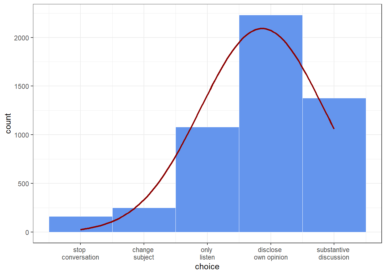

Appendix 1: Distribution of dependent variable

# fsave(appendix1)

6 Sample selection

Unique respondents before selection:

length(unique(df_sb2$crespnr))

#> [1] 1514

# delete respondents if missings on the two observations for the dependent!
table(is.na(df_sb2$L1), is.na(df_sb2$L2))
df_sb2 <- df_sb2[!is.na(df_sb2$L1) & !is.na(df_sb2$L2), ]  #266

# delete if missing on main independent vars: gender, ethnicity, age, acquaintanceship network

# gender
table(df_sb2$female, useNA = "always")  #0

# ethnicity
table(df_sb2$egoO, useNA = "always")  #12

# age
table(is.na(df_sb2$cage))  #age: 2

# educ
table(is.na(df_sb2$C05))  #educ: 0

# network
table(is.na(df_sb2$netsover3), useNA = "always")  #98

# listwise deletion
df_sb2 <- df_sb2[!is.na(df_sb2$egoO) & !is.na(df_sb2$cage) & !is.na(df_sb2$netsover3), ]


# #missings additional controls (no listwise deletion, these controls only in robustness)
# table(is.na(df_sb2$H19i))#thermoN: 166 table(is.na(df_sb2$H19j))#thermoN: 129
# table(is.na(df_sb2$H19k))#thermoN: 118 table(is.na(df_sb2$ego_opinion1)) # 3
# table(is.na(df_sb2$ego_opinion1b)) table(is.na(df_sb2$ego_opinion2))#: 3
# table(is.na(df_sb2$ego_opinion3))# 0 table(is.na(df_sb2$H06)) #political interest: 0 #district
# vars table(is.na(df_sb2$district_EI_ethnic))

#>        
#>         FALSE TRUE
#>   FALSE  1242    4
#>   TRUE      2  266
#> 
#>    0    1 <NA> 
#>  591  651    0 
#> 
#>    0    1 <NA> 
#> 1230   12    0 
#> 
#> FALSE  TRUE 
#>  1240     2 
#> 
#> FALSE 
#>  1242 
#> 
#> FALSE  TRUE  <NA> 
#>  1144    98     0

Unique respondents after selection:

length(unique(df_sb2$crespnr))  #1143

#> [1] 1143

7 Table 3

Descriptive statistics working sample (split ballot 2).

select2 <- c("female", "egoNL", "egoM", "egoT", "netsover3", "hhi_gender", "hhi_ethnic", "cage", "educL",
    "educM", "educH")


df_sel2 <- df_sb2[, select2]
table_des <- psych::describe(df_sel2)
table_des$missing <- colSums(is.na(df_sel2))
table3 <- table_des %>%
    mutate(variable = rownames(table_des)) %>%
    select(variable, mean, sd, min, max) %>%
    flextable() %>%
    set_caption("Table 3. Descriptive statistics independent variables (respondent-level)") %>%
    colformat_double(j = c("min", "max"), digits = c(0), big.mark = "") %>%
    colformat_double(j = c("mean", "sd"), digits = c(3), big.mark = "") %>%
    colformat_double(i = c(6, 7), j = c("min", "max"), digits = c(3), big.mark = "") %>%
    set_header_labels(mean = "mean / \nproportion") %>%
    mk_par(j = 1, value = as_paragraph(c("Women", "Ethnicity \n\n \t Native-Dutch", "\t Moroccan-Dutch",
        "\t Turkish-Dutch", "Network size", "Network gender diversity", "Network ethnic diversity", "Age",
        "Education \n\n \t Primary", "\t Secondary", "\t Tertiary"))) %>%
    valign(valign = "bottom", part = "body") %>%
    width(j = 1, width = 60, unit = "mm") %>%
    add_footer_row(values = c("N = 1,143"), colwidths = 5)
table3
# fsave(table3)

Table 3. Descriptive statistics independent variables (respondent-level)
variable	mean / proportion	sd	min	max
Women	0.529	0.499	0	1
Ethnicity Native-Dutch	0.610	0.488	0	1
Moroccan-Dutch	0.144	0.352	0	1
Turkish-Dutch	0.239	0.427	0	1
Network size	532.579	348.162	89	2691
Network gender diversity	0.407	0.139	0.000	0.500
Network ethnic diversity	0.307	0.232	0.000	0.667
Age	31.857	8.815	16	55
Education Primary	0.146	0.353	0	1
Secondary	0.382	0.486	0	1
Tertiary	0.472	0.499	0	1
N = 1,143

8 Multivariate analyses

Dutch description of vignette.

Module L: Vignette Er volgen nu twee verschillende situaties over politieke gesprekken. We vragen u om zich in deze situatie in te beelden. We zijn benieuwd naar wat u zou doen.

We begrijpen dat de situaties mogelijk niet (vaak) voorkomen in uw dagelijks leven. Probeer de vraag toch te beantwoorden.

L1: Stelt u zich voor dat u een {e://Field/gender1} van {e://Field/groep1} afkomst tegenkomt. Dit zou bijvoorbeeld kunnen zijn op straat, het openbaar vervoer, op uw werk, of bij een (sport)vereniging. Deze persoon is {e://Field/relatie1}. Deze persoon knoopt met u een praatje aan.

Na een tijdje komt het recente politieke voorstel ter sprake om {e://Field/issue1}. Het wordt duidelijk dat deze persoon {e://Field/positie1}.

Wat doet u?

Ik stop het gesprek.
Ik probeer het gesprek op een ander onderwerp te krijgen.
Ik luister naar de ander: Ik geef niet mijn eigen mening en vermijd een inhoudelijke discussie.
Ik ga in gesprek: Ik geef mijn eigen mening, maar vermijd een inhoudelijke discussie.
Ik ga in discussie: Ik geef mijn eigen mening en bespreek argumenten voor en tegen.

L2: Stelt u zich voor dat u een {e://Field/gender2} van {e://Field/groep2} afkomst tegenkomt. Dit zou bijvoorbeeld kunnen zijn op straat, het openbaar vervoer, op uw werk, of bij een (sport)vereniging. Deze persoon is ${e://Field/relatie2}. Deze persoon knoopt met u een praatje aan.

Na een tijdje komt het recente politieke voorstel ter sprake om {e://Field/issue2}. Het wordt duidelijk dat deze persoon ${e://Field/positie2}.

Wat doet u?

Ik stop het gesprek.
Ik probeer het gesprek op een ander onderwerp te krijgen.
Ik luister naar de ander: Ik geef niet mijn eigen mening en vermijd een inhoudelijke discussie.
Ik ga in gesprek: Ik geef mijn eigen mening, maar vermijd een inhoudelijke discussie.
Ik ga in discussie: Ik geef mijn eigen mening en bespreek argumenten voor en tegen.

Vignette dimensies: Gender: 1. Man 2. Vrouw Groep: 1. Marokkaanse 2. Nederlandse 3. Turkse Relatie 1. een collega 2. een goede vriend(in) 3. een kennis 4. familie (aangetrouwd) 5. iemand die je net bent tegengekomen Issue: 1. hogere belastingen voor mensen met topinkomens in te voeren 2. minder vluchtelingen op te nemen in Nederland 3. subsidies op maatregelen die duurzaamheid vergroten (bijvoorbeeld elektrische auto’s, zonnepanelen en warmtepompen) af te bouwen Positie 1. een stuk negatiever denkt over dit voorstel dan u 2. een stuk positiever denkt over dit voorstel dan u 3. ongeveer hetzelfde denkt over dit voorstel als u

8.1 Nested linear

We nest the observations within the respondent-level.

select <- c("crespnr", "L1", "L2", "cL1_gender", "cL2_gender", "cL1_relatie", "cL2_relatie", "cL1_issue",
    "cL2_issue", "cL1_positie", "cL2_positie", "cL1_groep", "cL2_groep", "female", "egoNL", "egoM", "egoT",
    "ego_gen1", "cage", "educL", "educM", "educH", "educ_current", "thermoD", "thermoM", "thermoT", "ego_opinion1",
    "ego_opinion2", "ego_opinion3", "polint", "cdn_tot", "cdn_tot_nk", "cdn_EI_ethnic", "cdn_EI_gender",
    "netsover3", "nsum_EI_ethnic", "nsum_EI_gender", "hhi_educ", "hhi_gender", "hhi_ethnic", "district_EI_ethnic",
    "district_EI_gender")

df_sel <- df_sb2[, select]


df1 <- df_sel
df2 <- df_sel
df1$index <- 1
df2$index <- 2
df_tot <- rbind(df1, df2)

df_tot$Y_L <- ifelse(df_tot$index == 1, df_tot$L1, df_tot$L2)
df_tot$L_gender <- ifelse(df_tot$index == 1, df_tot$cL1_gender, df_tot$cL2_gender)
df_tot$L_relatie <- ifelse(df_tot$index == 1, df_tot$cL1_relatie, df_tot$cL2_relatie)
df_tot$L_issue <- ifelse(df_tot$index == 1, df_tot$cL1_issue, df_tot$cL2_issue)
df_tot$L_positie <- ifelse(df_tot$index == 1, df_tot$cL1_positie, df_tot$cL2_positie)
df_tot$L_groep <- ifelse(df_tot$index == 1, df_tot$cL1_groep, df_tot$cL2_groep)

We recode position for issue1 so in same ‘right-wing’ direction. So for position, more positive means more ‘right-wing’.

df_tot <- df_tot %>%
    mutate(L_positie = case_when(L_issue == 1 ~ case_match(L_positie, 1 ~ 2, 2 ~ 1, 3 ~ 3), .default = L_positie))

We match the political opinion of the respondent to the correct policy measure/issue as presented in the vignette. We do not use this in the main manuscript.

df_tot <- df_tot %>%
    mutate(ego_opinion = case_when(L_issue == 1 ~ ego_opinion1, .default = NA), ego_opinion = case_when(L_issue ==
        2 ~ ego_opinion2, .default = ego_opinion), ego_opinion = case_when(L_issue == 3 ~ ego_opinion3,
        .default = ego_opinion))

We change some reference categories.

df_tot$L_groep <- relevel(as.factor(df_tot$L_groep), 2)  #dutch ref
df_tot$L_positie <- relevel(as.factor(df_tot$L_positie), 3)  #same ref

We bin some categories in the relation dimension into ‘weak’ and ‘strong’ ties.

# attributes(df_tot$cL1_relatie)

df_tot <- df_tot %>%
    mutate(L_relatie2 = case_match(L_relatie, c(1, 3, 5) ~ "weak", c(2, 4) ~ "strong"))

Similarly we bin categories in the political distance dimension into ‘same’ and ‘different’.

# attributes(df_tot$cL1_positie)
df_tot <- df_tot %>%
    mutate(L_positie2 = case_match(L_positie, c("1", "2") ~ "different", c("3") ~ "same"))

Dyadic similarity measures

Dyadic similarity is based on ego’s characteristics and the characteristic of alter, as described in the vignette.

df_tot <- df_tot %>%
    mutate(gen_sim = case_when((L_gender == 1 & female == 0) | (L_gender == 2 & female == 1) ~ 1, .default = 0),
        ethnic_sim = case_when((L_groep == 1 & egoM == 1) | (L_groep == 2 & egoNL == 1) | (L_groep ==
            3 & egoT == 1) ~ 1, .default = 0))

Or our robustness analysis per ethnic group we think it is more intuitive to construct a dyadic variable indicating whether the alter belongs to an ethnic/gender outgroup.

df_tot <- df_tot %>%
    mutate(outgroup = case_when((L_groep == 1 & egoNL == 1) | (L_groep == 3 & egoNL == 1) ~ 1, (L_groep ==
        2 & egoM == 1) | (L_groep == 3 & egoM == 1) ~ 1, (L_groep == 1 & egoT == 1) | (L_groep == 2 &
        egoT == 1) ~ 1, .default = 0))

We will fit models with the R package lme4 (Bates et al. 2015). From past experience, we know reviewers like p-values. However, there is a reason why in lmer p-values are not reported by default: [(https://stat.ethz.ch/pipermail/r-help/2006-May/094765.html)]. We use the R package jtools (Long 2022) for these purposes. Perhaps better is to report CI.

8.2 Overview hypotheses

the likelihood of political talk increases when potential discussion partners share a (a) gender, (b) ethnic background, or (c) congruent political views (H1).
the likelihood of political talk increases when potential discussion partners are strong rather than weak ties (H2).
the positive effect of (a) gender and (b) ethnic background similarity between potential discussion partners on political talk increases when discussion partners are weak (i.e., colleagues, acquaintances) rather than strong ties (i.e., good friends, family members) (H3).
individuals with larger acquaintanceship networks are more likely to engage in political talk (H4).
individuals with more (a) gender and (b) ethnically diverse acquaintanceship networks are more likely to engage in political talk (H5).
1. the positive effect of gender background similarity between potential discussion partners on political talk decreases when the respondent’s network is more gender diverse; (b) the positive effect of ethnic background similarity between potential discussion partners on political talk decreases when the respondent’s network is more ethnically diverse;

# Model empty in appendix?
M_empty <- (lmer(Y_L ~ +(1 | crespnr), data = df_tot))


# Model 0 in appendix?
M0 <- (lmer(Y_L ~ as.factor(L_gender) + as.factor(L_groep) + as.factor(L_relatie) + as.factor(L_issue) +
    as.factor(L_positie) + as.factor(L_groep) + (1 | crespnr), data = df_tot))

# hypo1 / hypo2
M1 <- lmer(Y_L ~ as.factor(L_gender) + as.factor(L_groep) + as.factor(L_relatie2) + as.factor(L_issue) +
    as.factor(L_positie2) + female + egoM + egoT + gen_sim + ethnic_sim + cage + educM + educH + (1 |
    crespnr), data = df_tot)

# hypo3
M2 <- lmer(Y_L ~ as.factor(L_gender) + as.factor(L_groep) + as.factor(L_relatie2) + as.factor(L_issue) +
    as.factor(L_positie2) + female + egoM + egoT + gen_sim + ethnic_sim + cage + educM + educH + as.factor(L_relatie2) *
    gen_sim + as.factor(L_relatie2) * ethnic_sim + as.factor(L_relatie2) * as.factor(L_positie2) + (1 |
    crespnr), data = df_tot)


# hypo 4 / 5 M3_alt <- lmer(Y_L ~ as.factor(L_gender) + as.factor(L_relatie2) + as.factor(L_issue)
# + as.factor(L_positie2) + as.factor(L_groep) + female + egoM + egoT + gen_sim + ethnic_sim + cage
# + educM + educH + log(netsover3) + hhi_gender + hhi_ethnic + cage + educM + educH + (1 |
# crespnr), data=df_tot )

M3 <- lmer(Y_L ~ as.factor(L_gender) + as.factor(L_groep) + as.factor(L_relatie2) + as.factor(L_issue) +
    as.factor(L_positie2) + as.factor(L_groep) + female + egoM + egoT + gen_sim + ethnic_sim + cage +
    educM + educH + log(netsover3) + hhi_gender + hhi_ethnic + as.factor(L_relatie2) * gen_sim + as.factor(L_relatie2) *
    ethnic_sim + as.factor(L_relatie2) * as.factor(L_positie2) + (1 | crespnr), data = df_tot)

# based on suggestion reviewer, without family members
M3_RR1 <- lmer(Y_L ~ as.factor(L_gender) + as.factor(L_groep) + as.factor(L_relatie2) + as.factor(L_issue) +
    as.factor(L_positie2) + as.factor(L_groep) + female + egoM + egoT + gen_sim + ethnic_sim + cage +
    educM + educH + log(netsover3) + hhi_gender + hhi_ethnic + as.factor(L_relatie2) * gen_sim + as.factor(L_relatie2) *
    ethnic_sim + as.factor(L_relatie2) * as.factor(L_positie2) + (1 | crespnr), data = df_tot[df_tot$L_relatie !=
    4, ])
# summary(M3_RR1)



M4 <- lmer(Y_L ~ as.factor(L_gender) + as.factor(L_groep) + as.factor(L_relatie2) + as.factor(L_issue) +
    as.factor(L_positie2) + as.factor(L_groep) + female + egoM + egoT + gen_sim + ethnic_sim + cage +
    educM + educH + as.factor(L_relatie2) * gen_sim + as.factor(L_relatie2) * ethnic_sim + as.factor(L_relatie2) *
    as.factor(L_positie2) + log(netsover3) + hhi_gender + hhi_ethnic + gen_sim * hhi_gender + gen_sim *
    hhi_ethnic + cage + educM + educH + (1 | crespnr), data = df_tot)

pvalue_format <- function(x) {
    # p <- 2*pt(q=x, df=1000, lower.tail=FALSE)
    z <- cut(x, breaks = c(-Inf, 0.001, 0.01, 0.05, 0.1, Inf), labels = c("***", "**", "*", "~", ""))
    as.character(z)
}

df_M0 <- as_tibble(summ(M0)$coeftable) %>%
    mutate(terms = rownames(summ(M0)$coeftable), sig = pvalue_format(p)) %>%
    select(c("terms", "Est.", "sig", "S.E."))

df_M1 <- as_tibble(summ(M1)$coeftable) %>%
    mutate(terms = rownames(summ(M1)$coeftable), sig = pvalue_format(p)) %>%
    select(c("terms", "Est.", "sig", "S.E."))

df_M2 <- as_tibble(summ(M2)$coeftable) %>%
    mutate(terms = rownames(summ(M2)$coeftable), sig = pvalue_format(p)) %>%
    select(c("terms", "Est.", "sig", "S.E."))

df_M3 <- as_tibble(summ(M3)$coeftable) %>%
    mutate(terms = rownames(summ(M3)$coeftable), sig = pvalue_format(p)) %>%
    select(c("terms", "Est.", "sig", "S.E."))

df_M4 <- as_tibble(summ(M4)$coeftable) %>%
    mutate(terms = rownames(summ(M4)$coeftable), sig = pvalue_format(p)) %>%
    select(c("terms", "Est.", "sig", "S.E."))

df_models <- full_join(df_M1, df_M2, by = c("terms")) %>%
    full_join(y = df_M3, by = c("terms")) %>%
    full_join(y = df_M4, by = c("terms"))

8.3 Appendix 2

We report the null-model (original categories vignette, no other covariates) in Appendix 2 of the manuscript.

vars_empty <- as.data.frame(VarCorr(M_empty))
# summary(M0)
vars <- as.data.frame(VarCorr(M0))
# round(vars$vcov,3)

appendix2 <- df_M0 %>%
    flextable() %>%
    add_header_row(values = c(" ", c("Estimate", " ", "Std.Error")), top = FALSE) %>%
    delete_rows(i = 1, part = "header") %>%
    align(i = 1, align = "center", part = "header") %>%
    align(j = 3, align = "left") %>%
    padding(padding.left = 0, j = c(3), part = "all") %>%
    padding(padding.right = 0, j = c(2), part = "all") %>%
    valign(valign = "bottom", part = "body") %>%
    width(j = 1, width = 60, unit = "mm") %>%
    mk_par(j = 1, value = as_paragraph(c("Intercept", "Alter gender (men = ref.) \n\n\t woman", "Ethnic background alter (native Dutch = ref.) \n\n\t Moroccan",
        "\t Turkish", "Relationship type (colleague = ref.) \n\n\t friend", "\t acquaintance", "\t family",
        "\t stranger", "Policy (higher tax for high incomes = ref.) \n\n\t less refugees", "\t reduce climate subsidies",
        "Political distance (similar = ref.) \n\n\t more negative", "\t more positive"))) %>%
    colformat_double(j = c(2, 4), digits = 3) %>%
    add_body_row(values = c("R^2_resp.", round(100 * (vars_empty$vcov[1] - vars$vcov[1])/vars_empty$vcov[1],
        3)), colwidths = c(1, 3), top = FALSE) %>%
    add_body_row(values = c("R^2_obs.", round(100 * (vars_empty$vcov[2] - vars$vcov[2])/vars_empty$vcov[2],
        3)), colwidths = c(1, 3), top = FALSE) %>%
    align(i = c(13, 14), j = c(2:4), align = "center", part = "body") %>%
    border_inner_h(border = fp_border_default(width = 0), part = "body") %>%
    hline(i = 12) %>%
    add_footer_lines(value = c("***p<.001, **p<.01, *p<.05, ~p<.10")) %>%
    add_footer_lines(value = c("N_obs = 2,286; N_resp = 1,142")) %>%
    fontsize(size = 8, part = "all") %>%
    set_table_properties(layout = "autofit")

appendix2 %>%
    set_caption("Appendix 2: predicting political talk with vignette characteristics only")
# fsave(appendix2)

Appendix 2: predicting political talk with vignette characteristics only
	Estimate		Std.Error
Intercept	3.922	***	0.057
Alter gender (men = ref.) woman	-0.000		0.030
Ethnic background alter (native Dutch = ref.) Moroccan	-0.084	*	0.036
Turkish	-0.061	~	0.036
Relationship type (colleague = ref.) friend	0.112	*	0.048
acquaintance	0.046		0.048
family	0.060		0.048
stranger	-0.000		0.048
Policy (higher tax for high incomes = ref.) less refugees	-0.033		0.036
reduce climate subsidies	0.015		0.036
Political distance (similar = ref.) more negative	-0.057		0.036
more positive	0.028		0.037
R^2_resp.	0.04
R^2_obs.	0.673
*p<.001, p<.01, *p<.05, ~p<.10
N_obs = 2,286; N_resp = 1,142

8.4 Table 4

varsm1 <- as.data.frame(VarCorr(M1))
varsm2 <- as.data.frame(VarCorr(M2))
varsm3 <- as.data.frame(VarCorr(M3))
varsm4 <- as.data.frame(VarCorr(M4))

table4 <- df_models %>%
    flextable() %>%
    add_header_row(values = c(" ", rep(c("Estimate", " ", "Std.Error"), 4)), top = FALSE) %>%
    delete_rows(i = 1, part = "header") %>%
    add_header_row(values = c(" ", "Model 1", "Model 2", "Model 3", "Model 4"), colwidths = c(1, 3, 3,
        3, 3)) %>%
    align(i = 1, align = "center", part = "header") %>%
    align(j = c(3, 6, 9, 12), align = "left") %>%
    padding(padding.left = 0, j = c(3, 6, 9, 12), part = "all") %>%
    padding(padding.right = 0, j = c(2, 5, 8, 11), part = "all") %>%
    mk_par(j = 1, value = as_paragraph(c("Intercept", "Gender alter (men = ref.) \n\n\t woman", "Ethnic background alter (native Dutch = ref.) \n\n\t Moroccan",
        "\t Turkish", "Tie strength (strong = ref.) \n\n\t weak", "Policy (higher tax for high incomes = ref.) \n\n\t less refugees",
        "\t reduce climate subsidies", "Political distance (different = ref.) \n\n\t similar", "Gender ego (men =ref.) \n\n\t woman",
        "Ethnic background ego (native Dutch = ref.) \n\n\t Moroccan", "\t Turkish", "Gender similarity dyad",
        "Ethnic similarity dyad", "Age ego", "Education ego (primary =ref.) \n\n\t secondary", "\t tertiary",
        "Weak tie * gender similarity", "Weak tie * ethnic similarity", "Weak tie * opinion similarity",
        "Network size", "Network gender diversity", "Network ethnic diversity", "Gender similarity * gender diversity",
        "Ethnic similarity * ethnic diversity"))) %>%
    valign(valign = "bottom", part = "body") %>%
    width(j = 1, width = 60, unit = "mm") %>%
    add_footer_lines(value = c("***p<.001, **p<.01, *p<.05, ~p<.10")) %>%
    add_footer_lines(value = c("N_obs = 2,286; N_resp = 1,142")) %>%
    colformat_double(digits = 3) %>%
    add_body_row(values = c("var_resp.", c(round(varsm1$vcov, 3)[1], round(varsm2$vcov, 3)[1], round(varsm3$vcov,
        3)[1], round(varsm4$vcov, 3)[1])), colwidths = c(1, 3, 3, 3, 3), top = FALSE) %>%
    add_body_row(values = c("var_obs.", c(round(varsm1$vcov, 3)[2], round(varsm2$vcov, 3)[2], round(varsm3$vcov,
        3)[2], round(varsm4$vcov, 3)[2])), colwidths = c(1, 3, 3, 3, 3), top = FALSE) %>%
    align(i = c(25, 26), j = c(2:13), align = "center", part = "body") %>%
    border_inner_h(border = fp_border_default(width = 0), part = "body") %>%
    hline(i = 24) %>%
    fontsize(size = 8, part = "all") %>%
    set_table_properties(layout = "autofit")

table4 %>%
    set_caption("Table 4. Willingness to talk politics")
# fsave(table4)

Table 4. Willingness to talk politics
	Model 1			Model 2			Model 3			Model 4
	Estimate		Std.Error	Estimate		Std.Error	Estimate		Std.Error	Estimate		Std.Error
Intercept	3.729	***	0.122	3.794	***	0.124	3.901	***	0.325	3.946	***	0.329
Gender alter (men = ref.) woman	-0.001		0.030	-0.001		0.030	-0.001		0.030	0.005		0.030
Ethnic background alter (native Dutch = ref.) Moroccan	-0.059		0.040	-0.061		0.040	-0.061		0.040	-0.063		0.040
Turkish	-0.048		0.039	-0.044		0.039	-0.044		0.039	-0.045		0.039
Tie strength (strong = ref.) weak	-0.069	*	0.030	-0.185	***	0.051	-0.186	***	0.051	-0.184	***	0.051
Policy (higher tax for high incomes = ref.) less refugees	-0.031		0.036	-0.036		0.036	-0.037		0.036	-0.036		0.036
reduce climate subsidies	0.014		0.036	0.018		0.036	0.015		0.036	0.017		0.036
Political distance (different = ref.) similar	0.016		0.032	-0.048		0.049	-0.050		0.049	-0.049		0.049
Gender ego (men =ref.) woman	-0.246	***	0.052	-0.246	***	0.052	-0.249	***	0.052	-0.248	***	0.052
Ethnic background ego (native Dutch = ref.) Moroccan	0.096		0.076	0.089		0.076	-0.016		0.085	-0.016		0.086
Turkish	-0.046		0.062	-0.049		0.062	-0.146	*	0.073	-0.146	*	0.073
Gender similarity dyad	0.045		0.030	-0.048		0.046	-0.045		0.046	-0.128		0.097
Ethnic similarity dyad	0.028		0.035	0.040		0.051	0.041		0.051	0.044		0.051
Age ego	-0.000		0.003	-0.000		0.003	-0.001		0.003	-0.001		0.003
Education ego (primary =ref.) secondary	0.305	***	0.080	0.305	***	0.080	0.311	***	0.080	0.306	***	0.080
tertiary	0.515	***	0.081	0.513	***	0.081	0.531	***	0.081	0.530	***	0.081
Weak tie * gender similarity				0.166	**	0.060	0.162	**	0.060	0.159	**	0.060
Weak tie * ethnic similarity				-0.010		0.064	-0.009		0.064	-0.013		0.064
Weak tie * opinion similarity				0.113	~	0.064	0.116	~	0.064	0.113	~	0.064
Network size							-0.046		0.052	-0.046		0.052
Network gender diversity							0.231		0.208	0.231		0.234
Network ethnic diversity							0.374	**	0.140	0.234		0.155
Gender similarity * gender diversity										-0.001		0.211
Ethnic similarity * ethnic diversity										0.275	*	0.129
var_resp.	0.61			0.606			0.602			0.604
var_obs.	0.294			0.293			0.293			0.292
*p<.001, p<.01, *p<.05, ~p<.10
N_obs = 2,286; N_resp = 1,142

8.4.1 without families as strong ties

An anonymous reviewer raised the question to what extent results are impacted by unrealistic scenario’s. In our opinion, only - or at least especially - scenarios involving family members may have been unrealistic. We therefore re-estimate model 0 and without family members.

8.4.1.1 Model 0

levels(df_tot$L_relatie)

# Model 0
M0_nofamily <- (lmer(Y_L ~ as.factor(L_gender) + as.factor(L_groep) + as.factor(L_relatie) + as.factor(L_issue) +
    as.factor(L_positie) + as.factor(L_groep) + (1 | crespnr), data = df_tot[df_tot$L_relatie != 4, ]))
summary(M0_nofamily)

vars <- as.data.frame(VarCorr(M0_nofamily))
# round(vars$vcov,3)

pvalue_format <- function(x) {
    # p <- 2*pt(q=x, df=1000, lower.tail=FALSE)
    z <- cut(x, breaks = c(-Inf, 0.001, 0.01, 0.05, 0.1, Inf), labels = c("***", "**", "*", "~", ""))
    as.character(z)
}

df_M0_nofamily <- as_tibble(summ(M0_nofamily)$coeftable) %>%
    mutate(terms = rownames(summ(M0_nofamily)$coeftable), sig = pvalue_format(p)) %>%
    select(c("terms", "Est.", "sig", "S.E."))

RR1 <- df_M0_nofamily %>%
    flextable() %>%
    add_header_row(values = c(" ", c("Estimate", " ", "Std.Error")), top = FALSE) %>%
    delete_rows(i = 1, part = "header") %>%
    align(i = 1, align = "center", part = "header") %>%
    align(j = 3, align = "left") %>%
    padding(padding.left = 0, j = c(3), part = "all") %>%
    padding(padding.right = 0, j = c(2), part = "all") %>%
    valign(valign = "bottom", part = "body") %>%
    width(j = 1, width = 60, unit = "mm") %>%
    mk_par(j = 1, value = as_paragraph(c("Intercept", "Alter gender (men = ref.) \n\n\t woman", "Ethnic background alter (native Dutch = ref.) \n\n\t Moroccan",
        "\t Turkish", "Relationship type (colleague = ref.) \n\n\t friend", "\t acquaintance", "\t stranger",
        "Policy (higher tax for high incomes = ref.) \n\n\t less refugees", "\t reduce climate subsidies",
        "Political distance (similar = ref.) \n\n\t more negative", "\t more positive"))) %>%
    colformat_double(j = c(2, 4), digits = 3) %>%
    add_body_row(values = c("var_resp.", round(vars$vcov[1], 3)), colwidths = c(1, 3), top = FALSE) %>%
    add_body_row(values = c("var_obs.", round(vars$vcov[2], 3)), colwidths = c(1, 3), top = FALSE) %>%
    align(i = c(12, 13), j = c(2:4), align = "center", part = "body") %>%
    border_inner_h(border = fp_border_default(width = 0), part = "body") %>%
    hline(i = 11) %>%
    add_footer_lines(value = c("***p<.001, **p<.01, *p<.05, ~p<.10")) %>%
    add_footer_lines(value = c("N_obs = 1,806; N_resp = 1,092")) %>%
    fontsize(size = 8, part = "all") %>%
    set_table_properties(layout = "autofit")

RR1 %>%
    set_caption("RR1: predicting political talk with vignette characteristics only (excluding vignettes involving family members")

#> NULL
#> Linear mixed model fit by REML ['lmerMod']
#> Formula: Y_L ~ as.factor(L_gender) + as.factor(L_groep) + as.factor(L_relatie) +  
#>     as.factor(L_issue) + as.factor(L_positie) + as.factor(L_groep) +      (1 | crespnr)
#>    Data: df_tot[df_tot$L_relatie != 4, ]
#> 
#> REML criterion at convergence: 4596.6
#> 
#> Scaled residuals: 
#>     Min      1Q  Median      3Q     Max 
#> -3.9621 -0.3341  0.0615  0.4031  3.2840 
#> 
#> Random effects:
#>  Groups   Name        Variance Std.Dev.
#>  crespnr  (Intercept) 0.6383   0.7989  
#>  Residual             0.2970   0.5450  
#> Number of obs: 1806, groups:  crespnr, 1092
#> 
#> Fixed effects:
#>                        Estimate Std. Error t value
#> (Intercept)            3.932109   0.064028  61.412
#> as.factor(L_gender)2  -0.005721   0.035557  -0.161
#> as.factor(L_groep)1   -0.078478   0.042863  -1.831
#> as.factor(L_groep)3   -0.066095   0.043417  -1.522
#> as.factor(L_relatie)2  0.116116   0.050609   2.294
#> as.factor(L_relatie)3  0.068284   0.050770   1.345
#> as.factor(L_relatie)5  0.023909   0.050324   0.475
#> as.factor(L_issue)2   -0.044314   0.042529  -1.042
#> as.factor(L_issue)3    0.040511   0.042953   0.943
#> as.factor(L_positie)1 -0.097372   0.042968  -2.266
#> as.factor(L_positie)2  0.002950   0.044329   0.067
#> 
#> Correlation of Fixed Effects:
#>               (Intr) as.fctr(L_g)2 as.fctr(L_g)1 as.fctr(L_g)3 as.fctr(L_r)2 as.fctr(L_r)3 a.(L_)5
#> as.fctr(L_g)2 -0.308                                                                              
#> as.fctr(L_g)1 -0.329 -0.003                                                                       
#> as.fctr(L_g)3 -0.375  0.002         0.493                                                         
#> as.fctr(L_r)2 -0.418  0.039        -0.022        -0.018                                           
#> as.fctr(L_r)3 -0.405  0.018        -0.036        -0.018         0.531                             
#> as.fct(L_)5   -0.405  0.038        -0.010         0.001         0.532         0.528               
#> as.fctr(L_s)2 -0.361  0.036         0.016         0.072        -0.024        -0.025        -0.001 
#> as.fctr(L_s)3 -0.351  0.019        -0.002         0.058         0.005         0.006        -0.007 
#> as.fctr(L_p)1 -0.373 -0.005         0.029         0.041         0.001         0.006        -0.038 
#> as.fctr(L_p)2 -0.346  0.000         0.009         0.061        -0.003         0.001        -0.046 
#>               as.fctr(L_s)2 as.fctr(L_s)3 as.fctr(L_p)1
#> as.fctr(L_g)2                                          
#> as.fctr(L_g)1                                          
#> as.fctr(L_g)3                                          
#> as.fctr(L_r)2                                          
#> as.fctr(L_r)3                                          
#> as.fct(L_)5                                            
#> as.fctr(L_s)2                                          
#> as.fctr(L_s)3  0.495                                   
#> as.fctr(L_p)1  0.035         0.031                     
#> as.fctr(L_p)2 -0.004        -0.025         0.524

RR1: predicting political talk with vignette characteristics only (excluding vignettes involving family members
	Estimate		Std.Error
Intercept	3.932	***	0.064
Alter gender (men = ref.) woman	-0.006		0.036
Ethnic background alter (native Dutch = ref.) Moroccan	-0.078	~	0.043
Turkish	-0.066		0.043
Relationship type (colleague = ref.) friend	0.116	*	0.051
acquaintance	0.068		0.051
stranger	0.024		0.050
Policy (higher tax for high incomes = ref.) less refugees	-0.044		0.043
reduce climate subsidies	0.041		0.043
Political distance (similar = ref.) more negative	-0.097	*	0.043
more positive	0.003		0.044
var_resp.	0.638
var_obs.	0.297
*p<.001, p<.01, *p<.05, ~p<.10
N_obs = 1,806; N_resp = 1,092

8.4.1.2 Model 3

# based on suggestion reviewer, without family members
M3_RR1 <- lmer(Y_L ~ as.factor(L_gender) + as.factor(L_groep) + as.factor(L_relatie2) + as.factor(L_issue) +
    as.factor(L_positie2) + as.factor(L_groep) + female + egoM + egoT + gen_sim + ethnic_sim + cage +
    educM + educH + log(netsover3) + hhi_gender + hhi_ethnic + as.factor(L_relatie2) * gen_sim + as.factor(L_relatie2) *
    ethnic_sim + as.factor(L_relatie2) * as.factor(L_positie2) + (1 | crespnr), data = df_tot[df_tot$L_relatie !=
    4, ])
# summary(M3_RR1)

vars <- as.data.frame(VarCorr(M3_RR1))

pvalue_format <- function(x) {
    # p <- 2*pt(q=x, df=1000, lower.tail=FALSE)
    z <- cut(x, breaks = c(-Inf, 0.001, 0.01, 0.05, 0.1, Inf), labels = c("***", "**", "*", "~", ""))
    as.character(z)
}

df_M3_RR1 <- as_tibble(summ(M3_RR1)$coeftable) %>%
    mutate(terms = rownames(summ(M3_RR1)$coeftable), sig = pvalue_format(p)) %>%
    select(c("terms", "Est.", "sig", "S.E."))

RR2 <- df_M3_RR1 %>%
    flextable() %>%
    add_header_row(values = c(" ", c("Estimate", " ", "Std.Error")), top = FALSE) %>%
    delete_rows(i = 1, part = "header") %>%
    align(i = 1, align = "center", part = "header") %>%
    align(j = 3, align = "left") %>%
    padding(padding.left = 0, j = c(3), part = "all") %>%
    padding(padding.right = 0, j = c(2), part = "all") %>%
    valign(valign = "bottom", part = "body") %>%
    width(j = 1, width = 60, unit = "mm") %>%
    mk_par(j = 1, value = as_paragraph(c("Intercept", "Gender alter (men = ref.) \n\n\t woman", "Ethnic background alter (native Dutch = ref.) \n\n\t Moroccan",
        "\t Turkish", "Tie strength (strong = ref.) \n\n\t weak", "Policy (higher tax for high incomes = ref.) \n\n\t less refugees",
        "\t reduce climate subsidies", "Political distance (different = ref.) \n\n\t similar", "Gender ego (men =ref.) \n\n\t woman",
        "Ethnic background ego (native Dutch = ref.) \n\n\t Moroccan", "\t Turkish", "Gender similarity dyad",
        "Ethnic similarity dyad", "Age ego", "Education ego (primary =ref.) \n\n\t secondary", "\t tertiary",
        "Network size", "Network gender diversity", "Network ethnic diversity", "Weak tie * gender similarity",
        "Weak tie * ethnic similarity", "Weak tie * opinion similarity"))) %>%
    valign(valign = "bottom", part = "body") %>%
    width(j = 1, width = 60, unit = "mm") %>%
    add_footer_lines(value = c("***p<.001, **p<.01, *p<.05, ~p<.10")) %>%
    add_footer_lines(value = c("N_obs = 1,806; N_resp = 1,092")) %>%
    colformat_double(digits = 3) %>%
    add_body_row(values = c("var_resp.", c(round(vars$vcov, 3)[1])), colwidths = c(1, 3), top = FALSE) %>%
    add_body_row(values = c("var_obs.", c(round(vars$vcov, 3)[2])), colwidths = c(1, 3), top = FALSE) %>%
    align(i = c(23, 24), j = c(2:3), align = "center", part = "body") %>%
    border_inner_h(border = fp_border_default(width = 0), part = "body") %>%
    hline(i = 22) %>%
    fontsize(size = 8, part = "all") %>%
    set_table_properties(layout = "autofit")

RR2 %>%
    set_caption("RR2: predicting political talk, Model 3 of Table 4 (excluding vignettes involving family members")

RR2: predicting political talk, Model 3 of Table 4 (excluding vignettes involving family members
	Estimate		Std.Error
Intercept	4.031	***	0.345
Gender alter (men = ref.) woman	-0.002		0.035
Ethnic background alter (native Dutch = ref.) Moroccan	-0.056		0.047
Turkish	-0.046		0.046
Tie strength (strong = ref.) weak	-0.195	**	0.068
Policy (higher tax for high incomes = ref.) less refugees	-0.047		0.042
reduce climate subsidies	0.044		0.043
Political distance (different = ref.) similar	0.016		0.075
Gender ego (men =ref.) woman	-0.284	***	0.055
Ethnic background ego (native Dutch = ref.) Moroccan	0.045		0.089
Turkish	-0.129	~	0.076
Gender similarity dyad	-0.089		0.070
Ethnic similarity dyad	0.059		0.077
Age ego	-0.002		0.003
Education ego (primary =ref.) secondary	0.330	***	0.084
tertiary	0.540	***	0.085
Network size	-0.071		0.055
Network gender diversity	0.430	~	0.223
Network ethnic diversity	0.326	*	0.148
Weak tie * gender similarity	0.200	*	0.081
Weak tie * ethnic similarity	-0.028		0.087
Weak tie * opinion similarity	0.035		0.087
var_resp.	0.59
var_obs.	0.298
*p<.001, p<.01, *p<.05, ~p<.10
N_obs = 1,806; N_resp = 1,092

8.5 Appendix 3

Dichotomous dependent variable:
1. active political talk (original cats 4 and 5)
2. avoiding political talk (original cats 1,2 and 3)

8.5.1 Logit

# Model 0 dichotomous
M0 <- (glmer((Y_L > 3) ~ as.factor(L_gender) + as.factor(L_groep) + as.factor(L_relatie) + as.factor(L_issue) +
    as.factor(L_positie) + as.factor(L_groep) + (1 | crespnr), control = glmerControl(optimizer = c("bobyqa")),
    family = binomial, data = df_tot))
# summary(M0) fsave(M0)

To reach convergence we rescaled our age variable!

# scale age
df_tot$cage_s <- scale(df_tot$cage)

# hypo1 / hypo2
M1 <- glmer((Y_L > 3) ~ as.factor(L_gender) + as.factor(L_groep) + as.factor(L_relatie2) + as.factor(L_issue) +
    as.factor(L_positie2) + female + egoM + egoT + gen_sim + ethnic_sim + cage_s + educM + educH + (1 |
    crespnr), control = glmerControl(optimizer = c("bobyqa"), optCtrl = list(maxfun = 1e+05)), family = binomial,
    data = df_tot)
# fsave(M1)

# hypo3
M2 <- glmer((Y_L > 3) ~ as.factor(L_gender) + as.factor(L_groep) + as.factor(L_relatie2) + as.factor(L_issue) +
    as.factor(L_positie2) + female + egoM + egoT + gen_sim + ethnic_sim + cage_s + educM + educH + as.factor(L_relatie2) *
    gen_sim + as.factor(L_relatie2) * ethnic_sim + as.factor(L_relatie2) * as.factor(L_positie2) + (1 |
    crespnr), control = glmerControl(optimizer = c("bobyqa"), optCtrl = list(maxfun = 1e+05)), family = binomial,
    data = df_tot)
# fsave(M2)

M3 <- glmer((Y_L > 3) ~ as.factor(L_gender) + as.factor(L_groep) + as.factor(L_relatie2) + as.factor(L_issue) +
    as.factor(L_positie2) + as.factor(L_groep) + female + egoM + egoT + gen_sim + ethnic_sim + cage_s +
    educM + educH + log(netsover3) + hhi_gender + hhi_ethnic + as.factor(L_relatie2) * gen_sim + as.factor(L_relatie2) *
    ethnic_sim + as.factor(L_relatie2) * as.factor(L_positie2) + (1 | crespnr), control = glmerControl(optimizer = c("bobyqa"),
    optCtrl = list(maxfun = 1e+05)), family = binomial, data = df_tot)
# fsave(M3)

M4 <- glmer((Y_L > 3) ~ as.factor(L_gender) + as.factor(L_groep) + as.factor(L_relatie2) + as.factor(L_issue) +
    as.factor(L_positie2) + as.factor(L_groep) + female + egoM + egoT + gen_sim + ethnic_sim + cage_s +
    educM + educH + as.factor(L_relatie2) * gen_sim + as.factor(L_relatie2) * ethnic_sim + as.factor(L_relatie2) *
    as.factor(L_positie2) + log(netsover3) + hhi_gender + hhi_ethnic + gen_sim * hhi_gender + ethnic_sim *
    hhi_ethnic + (1 | crespnr), control = glmerControl(optimizer = c("bobyqa"), optCtrl = list(maxfun = 1e+05)),
    family = binomial, data = df_tot)
# fsave(M4)

pvalue_format <- function(x) {
    # p <- 2*pt(q=x, df=1000, lower.tail=FALSE)
    z <- cut(x, breaks = c(-Inf, 0.001, 0.01, 0.05, 0.1, Inf), labels = c("***", "**", "*", "~", ""))
    as.character(z)
}

# df_M0 <- as_tibble(summ(M0)$coeftable) %>% mutate(terms = rownames(summ(M0)$coeftable), sig =
# pvalue_format(p)) %>% select(c('terms', 'Est.', 'sig' ,'S.E.'))

df_M1 <- as_tibble(summ(M1)$coeftable) %>%
    mutate(terms = rownames(summ(M1)$coeftable), sig = pvalue_format(p)) %>%
    select(c("terms", "Est.", "sig", "S.E."))

df_M2 <- as_tibble(summ(M2)$coeftable) %>%
    mutate(terms = rownames(summ(M2)$coeftable), sig = pvalue_format(p)) %>%
    select(c("terms", "Est.", "sig", "S.E."))

df_M3 <- as_tibble(summ(M3)$coeftable) %>%
    mutate(terms = rownames(summ(M3)$coeftable), sig = pvalue_format(p)) %>%
    select(c("terms", "Est.", "sig", "S.E."))

df_M4 <- as_tibble(summ(M4)$coeftable) %>%
    mutate(terms = rownames(summ(M4)$coeftable), sig = pvalue_format(p)) %>%
    select(c("terms", "Est.", "sig", "S.E."))

df_models <- full_join(df_M1, df_M2, by = c("terms")) %>%
    full_join(y = df_M3, by = c("terms")) %>%
    full_join(y = df_M4, by = c("terms"))

varsm1 <- as.data.frame(VarCorr(M1))
varsm2 <- as.data.frame(VarCorr(M2))
varsm3 <- as.data.frame(VarCorr(M3))
varsm4 <- as.data.frame(VarCorr(M4))

appendix3 <- df_models %>%
    flextable() %>%
    add_header_row(values = c(" ", rep(c("Estimate", " ", "Std.Error"), 4)), top = FALSE) %>%
    delete_rows(i = 1, part = "header") %>%
    add_header_row(values = c(" ", "Model 1", "Model 2", "Model 3", "Model 4"), colwidths = c(1, 3, 3,
        3, 3)) %>%
    align(i = 1, align = "center", part = "header") %>%
    align(j = c(3, 6, 9, 12), align = "left") %>%
    padding(padding.left = 0, j = c(3, 6, 9, 12), part = "all") %>%
    padding(padding.right = 0, j = c(2, 5, 8, 11), part = "all") %>%
    mk_par(j = 1, value = as_paragraph(c("Intercept", "Gender alter (men = ref.) \n\n\t woman", "Ethnic background alter (native Dutch = ref.) \n\n\t Moroccan",
        "\t Turkish", "Tie strength (strong = ref.) \n\n\t weak", "Policy (higher tax for high incomes = ref.) \n\n\t less refugees",
        "\t reduce climate subsidies", "Political distance (different = ref.) \n\n\t similar", "Gender ego (men =ref.) \n\n\t woman",
        "Ethnic background ego (native Dutch = ref.) \n\n\t Moroccan", "\t Turkish", "Gender similarity dyad",
        "Ethnic similarity dyad", "Age ego", "Education ego (primary =ref.) \n\n\t secondary", "\t tertiary",
        "Weak tie * gender similarity", "Weak tie * ethnic similarity", "Weak tie * opinion similarity",
        "Network size", "Network gender diversity", "Network ethnic diversity", "Gender similarity * gender diversity",
        "Ethnic similarity * ethnic diversity"))) %>%
    valign(valign = "bottom", part = "body") %>%
    width(j = 1, width = 60, unit = "mm") %>%
    add_footer_lines(value = c("***p<.001, **p<.01, *p<.05, ~p<.10")) %>%
    add_footer_lines(value = c("N_obs = 2,286; N_resp = 1,142")) %>%
    colformat_double(digits = 3) %>%
    add_body_row(values = c("var_resp.", c(round(varsm1$vcov, 3)[1], round(varsm2$vcov, 3)[1], round(varsm3$vcov,
        3)[1], round(varsm4$vcov, 3)[1])), colwidths = c(1, 3, 3, 3, 3), top = FALSE) %>%
    align(i = c(25), j = c(2:13), align = "center", part = "body") %>%
    border_inner_h(border = fp_border_default(width = 0), part = "body") %>%
    hline(i = 24) %>%
    fontsize(size = 8, part = "all") %>%
    set_table_properties(layout = "autofit")

appendix3 %>%
    set_caption("Appendix 3: predicting actively engaging in political talk")
# fsave(appendix3)

Appendix 3: predicting actively engaging in political talk
	Model 1			Model 2			Model 3			Model 4
	Estimate		Std.Error	Estimate		Std.Error	Estimate		Std.Error	Estimate		Std.Error
Intercept	6.415	***	0.866	6.825	***	0.906	6.261	*	2.506	6.546	*	2.576
Gender alter (men = ref.) woman	0.198		0.257	0.220		0.259	0.216		0.259	0.212		0.262
Ethnic background alter (native Dutch = ref.) Moroccan	-0.613	~	0.345	-0.615	~	0.349	-0.606	~	0.347	-0.853	*	0.385
Turkish	-0.452		0.341	-0.432		0.343	-0.432		0.341	-0.672	~	0.376
Tie strength (strong = ref.) weak	-0.591	*	0.258	-1.344	**	0.432	-1.357	**	0.431	-1.331	**	0.432
Policy (higher tax for high incomes = ref.) less refugees	-0.429		0.304	-0.482		0.309	-0.492		0.307	-0.503		0.309
reduce climate subsidies	-0.202		0.303	-0.180		0.307	-0.197		0.306	-0.223		0.308
Political distance (different = ref.) similar	1.167	***	0.294	0.638		0.458	0.611		0.456	0.633		0.460
Gender ego (men =ref.) woman	-0.870	*	0.403	-0.911	*	0.407	-0.947	*	0.415	-0.968	*	0.417
Ethnic background ego (native Dutch = ref.) Moroccan	0.505		0.591	0.465		0.598	0.032		0.672	-0.014		0.680
Turkish	0.182		0.474	0.186		0.477	-0.171		0.551	-0.196		0.556
Gender similarity dyad	0.201		0.257	-0.524		0.419	-0.507		0.416	-0.307		0.799
Ethnic similarity dyad	0.430		0.310	0.683		0.499	0.679		0.495	0.003		0.638
Age ego	0.044		0.206	0.045		0.208	0.057		0.211	0.065		0.212
Education ego (primary =ref.) secondary	1.232	~	0.663	1.258	~	0.672	1.327	~	0.690	1.350	~	0.698
tertiary	1.662	*	0.682	1.707	*	0.691	1.843	**	0.713	1.854	*	0.720
Weak tie * gender similarity				1.203	*	0.522	1.181	*	0.520	1.148	*	0.522
Weak tie * ethnic similarity				-0.349		0.600	-0.337		0.596	-0.416		0.604
Weak tie * opinion similarity				0.905		0.584	0.932		0.582	0.910		0.584
Network size							-0.042		0.410	-0.037		0.413
Network gender diversity							0.818		1.596	1.044		1.820
Network ethnic diversity							1.581		1.106	0.982		1.169
Gender similarity * gender diversity										-0.477		1.723
Ethnic similarity * ethnic diversity										2.260	~	1.351
R^2_resp.	106.696			105.378			101.221			102.285
*p<.001, p<.01, *p<.05, ~p<.10
N_obs = 2,286; N_resp = 1,142

8.5.2 AME weak/strong ties

# mean value in data
mean(df_tot$Y_L > 3)

# check predicted values
mean(lme4:::predict.merMod(M1, type = "response"))  #include all random effects

# check predicted values
mean(lme4:::predict.merMod(M1, type = "response", re.form = NA))  #not including random effects
# a huge difference, this already indicates that most of our variance is at the respondent level.

# as.data.frame(ranef(fm01ML))
mean(lme4:::predict.merMod(M1, type = "response", random.only = TRUE))
# this indeed gives indication that we have important random effects.

# define the new datasets (depends of course on the AME you are interested in. simply use the
# numerical approach for everything) we have a categorical variable.

# define datasets to avoid annoying factor behavior in predicting scores, make strong/weak ties a
# numeric variable
df_tot$strong <- as.numeric(df_tot$L_relatie2 == "strong")

dfplus <- dfmin <- df_tot
# add the increase/decrease to the variable
dfplus$strong <- 1
dfmin$strong <- 0

# re-estimate model with numeric variable.  hypo1 / hypo2
M1 <- glmer((Y_L > 3) ~ as.factor(L_gender) + as.factor(L_groep) + strong + as.factor(L_issue) + as.factor(L_positie2) +
    female + egoM + egoT + gen_sim + ethnic_sim + cage_s + educM + educH + (1 | crespnr), control = glmerControl(optimizer = c("bobyqa"),
    optCtrl = list(maxfun = 1e+05)), family = binomial, data = df_tot)

# quick check: yes, same results summary(M1)

p1 <- lme4:::predict.merMod(M1, type = "response", newdata = dfplus)
p0 <- lme4:::predict.merMod(M1, type = "response", newdata = dfmin)
ame <- mean(p1 - p0)
ame  #0.0288037

# define function
mySumm <- function(fit) {
    p1 <- (lme4:::predict.merMod(fit, type = "response", newdata = dfplus))
    p0 <- (lme4:::predict.merMod(fit, type = "response", newdata = dfmin))

    am <- p1 - p0
    mean(am)
}

# run bootstrapping for SE given the very large random effects at the individual-level I do not
# want to resample these. therefore
library(parallel)
par_cores <- detectCores() - 1  #don't understand why I only see 50% of CPU usage (16 cores, 22 logical processors)
par_cluster <- makeCluster(rep("localhost", par_cores), outfile = "log.txt")
clusterEvalQ(par_cluster, library("lme4"))
clusterExport(par_cluster, varlist = c("df_tot", "M1", "dfplus", "dfmin", "mySumm"))

# note paralles 'multicore' does not seem to work, so have set up a snow cluster.
bb <- bootMer(M1, mySumm, nsim = 1000, , use.u = TRUE, parallel = "snow", ncpus = par_cores, cl = par_cluster,
    verbose = TRUE, .progress = "txt")


bb
# fsave(bb)
stopCluster(cl = par_cluster)

#> 
#> PARAMETRIC BOOTSTRAP
#> 
#> 
#> Call:
#> bootMer(x = M1, FUN = mySumm, nsim = 1000, use.u = TRUE, verbose = TRUE, 
#>     .progress = "txt", parallel = "snow", ncpus = par_cores, 
#>     cl = par_cluster)
#> 
#> 
#> Bootstrap Statistics :
#>      original      bias    std. error
#> t1* 0.0288037 -0.00165424  0.01253412

8.5.3 LPM

# Model 0 dichotomous
M0 <- (lmer((Y_L > 3) ~ as.factor(L_gender) + as.factor(L_groep) + as.factor(L_relatie) + as.factor(L_issue) +
    as.factor(L_positie) + as.factor(L_groep) + (1 | crespnr), data = df_tot))
# summary(M0)

# scale age
df_tot$cage_s <- scale(df_tot$cage)

# hypo1 / hypo2
M1 <- lmer((Y_L > 3) ~ as.factor(L_gender) + as.factor(L_groep) + as.factor(L_relatie2) + as.factor(L_issue) +
    as.factor(L_positie2) + female + egoM + egoT + gen_sim + ethnic_sim + cage_s + educM + educH + (1 |
    crespnr), data = df_tot)

# hypo3
M2 <- lmer((Y_L > 3) ~ as.factor(L_gender) + as.factor(L_groep) + as.factor(L_relatie2) + as.factor(L_issue) +
    as.factor(L_positie2) + female + egoM + egoT + gen_sim + ethnic_sim + cage_s + educM + educH + as.factor(L_relatie2) *
    gen_sim + as.factor(L_relatie2) * ethnic_sim + as.factor(L_relatie2) * as.factor(L_positie2) + (1 |
    crespnr), data = df_tot)

M3 <- lmer((Y_L > 3) ~ as.factor(L_gender) + as.factor(L_groep) + as.factor(L_relatie2) + as.factor(L_issue) +
    as.factor(L_positie2) + as.factor(L_groep) + female + egoM + egoT + gen_sim + ethnic_sim + cage_s +
    educM + educH + log(netsover3) + hhi_gender + hhi_ethnic + as.factor(L_relatie2) * gen_sim + as.factor(L_relatie2) *
    ethnic_sim + as.factor(L_relatie2) * as.factor(L_positie2) + (1 | crespnr), data = df_tot)

M4 <- lmer((Y_L > 3) ~ as.factor(L_gender) + as.factor(L_groep) + as.factor(L_relatie2) + as.factor(L_issue) +
    as.factor(L_positie2) + as.factor(L_groep) + female + egoM + egoT + gen_sim + ethnic_sim + cage_s +
    educM + educH + as.factor(L_relatie2) * gen_sim + as.factor(L_relatie2) * ethnic_sim + as.factor(L_relatie2) *
    as.factor(L_positie2) + log(netsover3) + hhi_gender + hhi_ethnic + gen_sim * hhi_gender + ethnic_sim *
    hhi_ethnic + (1 | crespnr), data = df_tot)

pvalue_format <- function(x) {
    # p <- 2*pt(q=x, df=1000, lower.tail=FALSE)
    z <- cut(x, breaks = c(-Inf, 0.001, 0.01, 0.05, 0.1, Inf), labels = c("***", "**", "*", "~", ""))
    as.character(z)
}

# df_M0 <- as_tibble(summ(M0)$coeftable) %>% mutate(terms = rownames(summ(M0)$coeftable), sig =
# pvalue_format(p)) %>% select(c('terms', 'Est.', 'sig' ,'S.E.'))

df_M1 <- as_tibble(summ(M1)$coeftable) %>%
    mutate(terms = rownames(summ(M1)$coeftable), sig = pvalue_format(p)) %>%
    select(c("terms", "Est.", "sig", "S.E."))

df_M2 <- as_tibble(summ(M2)$coeftable) %>%
    mutate(terms = rownames(summ(M2)$coeftable), sig = pvalue_format(p)) %>%
    select(c("terms", "Est.", "sig", "S.E."))

df_M3 <- as_tibble(summ(M3)$coeftable) %>%
    mutate(terms = rownames(summ(M3)$coeftable), sig = pvalue_format(p)) %>%
    select(c("terms", "Est.", "sig", "S.E."))

df_M4 <- as_tibble(summ(M4)$coeftable) %>%
    mutate(terms = rownames(summ(M4)$coeftable), sig = pvalue_format(p)) %>%
    select(c("terms", "Est.", "sig", "S.E."))

df_models <- full_join(df_M1, df_M2, by = c("terms")) %>%
    full_join(y = df_M3, by = c("terms")) %>%
    full_join(y = df_M4, by = c("terms"))

varsm1 <- as.data.frame(VarCorr(M1))
varsm2 <- as.data.frame(VarCorr(M2))
varsm3 <- as.data.frame(VarCorr(M3))
varsm4 <- as.data.frame(VarCorr(M4))

appendix3_lpm <- df_models %>%
    flextable() %>%
    add_header_row(values = c(" ", rep(c("Estimate", " ", "Std.Error"), 4)), top = FALSE) %>%
    delete_rows(i = 1, part = "header") %>%
    add_header_row(values = c(" ", "Model 1", "Model 2", "Model 3", "Model 4"), colwidths = c(1, 3, 3,
        3, 3)) %>%
    align(i = 1, align = "center", part = "header") %>%
    align(j = c(3, 6, 9, 12), align = "left") %>%
    padding(padding.left = 0, j = c(3, 6, 9, 12), part = "all") %>%
    padding(padding.right = 0, j = c(2, 5, 8, 11), part = "all") %>%
    mk_par(j = 1, value = as_paragraph(c("Intercept", "Gender alter (men = ref.) \n\n\t woman", "Ethnic background alter (native Dutch = ref.) \n\n\t Moroccan",
        "\t Turkish", "Tie strength (strong = ref.) \n\n\t weak", "Policy (higher tax for high incomes = ref.) \n\n\t less refugees",
        "\t reduce climate subsidies", "Political distance (different = ref.) \n\n\t similar", "Gender ego (men =ref.) \n\n\t woman",
        "Ethnic background ego (native Dutch = ref.) \n\n\t Moroccan", "\t Turkish", "Gender similarity dyad",
        "Ethnic similarity dyad", "Age ego", "Education ego (primary =ref.) \n\n\t secondary", "\t tertiary",
        "Weak tie * gender similarity", "Weak tie * ethnic similarity", "Weak tie * opinion similarity",
        "Network size", "Network gender diversity", "Network ethnic diversity", "Gender similarity * gender diversity",
        "Ethnic similarity * ethnic diversity"))) %>%
    valign(valign = "bottom", part = "body") %>%
    width(j = 1, width = 60, unit = "mm") %>%
    add_footer_lines(value = c("***p<.001, **p<.01, *p<.05, ~p<.10")) %>%
    add_footer_lines(value = c("N_obs = 2,286; N_resp = 1,142")) %>%
    colformat_double(digits = 3) %>%
    add_body_row(values = c("R^2_resp.", c(round(varsm1$vcov, 3)[1], round(varsm2$vcov, 3)[1], round(varsm3$vcov,
        3)[1], round(varsm4$vcov, 3)[1])), colwidths = c(1, 3, 3, 3, 3), top = FALSE) %>%
    align(i = c(25), j = c(2:13), align = "center", part = "body") %>%
    add_body_row(values = c("R^2_obs.", c(round(varsm1$vcov, 3)[2], round(varsm2$vcov, 3)[2], round(varsm3$vcov,
        3)[2], round(varsm4$vcov, 3)[2])), colwidths = c(1, 3, 3, 3, 3), top = FALSE) %>%
    align(i = c(26), j = c(2:13), align = "center", part = "body") %>%
    border_inner_h(border = fp_border_default(width = 0), part = "body") %>%
    hline(i = 24) %>%
    fontsize(size = 8, part = "all") %>%
    set_table_properties(layout = "autofit")

appendix3_lpm
# not shown in manuscript fsave(appendix3_lpm)

Appendix 3b: LPM (not shown in manuscript)
	Model 1			Model 2			Model 3			Model 4
	Estimate		Std.Error	Estimate		Std.Error	Estimate		Std.Error	Estimate		Std.Error
Intercept	0.626	***	0.043	0.661	***	0.044	0.645	***	0.140	0.645	***	0.143
Gender alter (men = ref.) woman	0.009		0.015	0.010		0.015	0.010		0.015	0.010		0.015
Ethnic background alter (native Dutch = ref.) Moroccan	-0.027		0.021	-0.028		0.021	-0.028		0.020	-0.039	~	0.022
Turkish	-0.028		0.020	-0.025		0.020	-0.025		0.020	-0.036	~	0.022
Tie strength (strong = ref.) weak	-0.030	~	0.016	-0.093	***	0.026	-0.093	***	0.026	-0.092	***	0.026
Policy (higher tax for high incomes = ref.) less refugees	-0.028		0.019	-0.031		0.019	-0.032	~	0.019	-0.032	~	0.019
reduce climate subsidies	-0.001		0.019	0.001		0.019	-0.001		0.019	-0.001		0.019
Political distance (different = ref.) similar	0.049	**	0.016	0.005		0.025	0.004		0.025	0.003		0.025
Gender ego (men =ref.) woman	-0.085	***	0.024	-0.085	***	0.024	-0.086	***	0.024	-0.087	***	0.024
Ethnic background ego (native Dutch = ref.) Moroccan	0.064	~	0.035	0.060	~	0.035	0.015		0.039	0.014		0.039
Turkish	0.026		0.028	0.025		0.028	-0.015		0.033	-0.016		0.033
Gender similarity dyad	0.013		0.015	-0.030		0.024	-0.028		0.024	0.009		0.049
Ethnic similarity dyad	0.026		0.018	0.030		0.027	0.031		0.027	-0.003		0.037
Age ego	0.005		0.012	0.005		0.012	0.005		0.012	0.005		0.012
Education ego (primary =ref.) secondary	0.120	**	0.037	0.120	**	0.036	0.122	***	0.036	0.123	***	0.036
tertiary	0.174	***	0.037	0.172	***	0.037	0.181	***	0.037	0.180	***	0.037
Weak tie * gender similarity				0.076	*	0.031	0.074	*	0.031	0.073	*	0.031
Weak tie * ethnic similarity				-0.001		0.033	-0.001		0.033	-0.003		0.033
Weak tie * opinion similarity				0.077	*	0.033	0.078	*	0.033	0.078	*	0.033
Network size							-0.010		0.024	-0.010		0.024
Network gender diversity							0.105		0.095	0.151		0.109
Network ethnic diversity							0.160	*	0.064	0.128	~	0.068
Gender similarity * gender diversity										-0.089		0.108
Ethnic similarity * ethnic diversity										0.102		0.077
R^2_resp.	0.115			0.114			0.113			0.113
R^2_obs.	0.084			0.084			0.084			0.084
*p<.001, p<.01, *p<.05, ~p<.10
N_obs = 2,286; N_resp = 1,142

8.6 Appendix 4

We also performed ethnic sub-group analysis. Mostly to check whether dyadic ethnic dissimilarity (i.e. outgroup) and network ethnic diversity has the same impact across the main ethnic groups in our sample.

M4b_tot <- lmer(Y_L ~ as.factor(L_gender) + as.factor(outgroup) + as.factor(L_relatie2) + as.factor(L_issue) +
    as.factor(L_positie2) + female + egoM + egoT + gen_sim + cage + educM + educH + as.factor(L_relatie2) *
    gen_sim + as.factor(L_relatie2) * as.factor(outgroup) + as.factor(L_relatie2) * as.factor(L_positie2) +
    log(netsover3) + hhi_gender + hhi_ethnic + gen_sim * hhi_gender + as.factor(outgroup) * hhi_ethnic +
    (1 | crespnr), data = df_tot)

M4b_NL <- lmer(Y_L ~ as.factor(L_gender) + as.factor(outgroup) + as.factor(L_relatie2) + as.factor(L_issue) +
    as.factor(L_positie2) + as.factor(outgroup) + female + gen_sim + cage + educM + educH + as.factor(L_relatie2) *
    gen_sim + as.factor(L_relatie2) * as.factor(outgroup) + as.factor(L_relatie2) * as.factor(L_positie2) +
    log(netsover3) + hhi_gender + hhi_ethnic + gen_sim * hhi_gender + as.factor(outgroup) * hhi_ethnic +
    (1 | crespnr), data = df_tot[df_tot$egoNL == 1, ])


M4b_M <- lmer(Y_L ~ as.factor(L_gender) + as.factor(outgroup) + as.factor(L_relatie2) + as.factor(L_issue) +
    as.factor(L_positie2) + as.factor(outgroup) + female + gen_sim + cage + educM + educH + as.factor(L_relatie2) *
    gen_sim + as.factor(L_relatie2) * as.factor(outgroup) + as.factor(L_relatie2) * as.factor(L_positie2) +
    log(netsover3) + hhi_gender + hhi_ethnic + gen_sim * hhi_gender + as.factor(outgroup) * hhi_ethnic +
    (1 | crespnr), data = df_tot[df_tot$egoM == 1, ])

M4b_T <- lmer(Y_L ~ as.factor(L_gender) + as.factor(outgroup) + as.factor(L_relatie2) + as.factor(L_issue) +
    as.factor(L_positie2) + as.factor(outgroup) + female + gen_sim + cage + educM + educH + as.factor(L_relatie2) *
    gen_sim + as.factor(L_relatie2) * as.factor(outgroup) + as.factor(L_relatie2) * as.factor(L_positie2) +
    log(netsover3) + hhi_gender + hhi_ethnic + gen_sim * hhi_gender + as.factor(outgroup) * hhi_ethnic +
    (1 | crespnr), data = df_tot[df_tot$egoT == 1, ])

pvalue_format <- function(x) {
    # p <- 2*pt(q=x, df=1000, lower.tail=FALSE)
    z <- cut(x, breaks = c(-Inf, 0.001, 0.01, 0.05, 0.1, Inf), labels = c("***", "**", "*", "~", ""))
    as.character(z)
}

df_M4b <- as_tibble(summ(M4b_tot)$coeftable) %>%
    mutate(terms = rownames(summ(M4b_tot)$coeftable), sig = pvalue_format(p)) %>%
    select(c("terms", "Est.", "sig", "S.E."))

df_M4b_NL <- as_tibble(summ(M4b_NL)$coeftable) %>%
    mutate(terms = rownames(summ(M4b_NL)$coeftable), sig = pvalue_format(p)) %>%
    select(c("terms", "Est.", "sig", "S.E."))

df_M4b_M <- as_tibble(summ(M4b_M)$coeftable) %>%
    mutate(terms = rownames(summ(M4b_M)$coeftable), sig = pvalue_format(p)) %>%
    select(c("terms", "Est.", "sig", "S.E."))

df_M4b_T <- as_tibble(summ(M4b_T)$coeftable) %>%
    mutate(terms = rownames(summ(M4b_T)$coeftable), sig = pvalue_format(p)) %>%
    select(c("terms", "Est.", "sig", "S.E."))


dfM4b <- full_join(df_M4b, df_M4b_NL, by = c("terms")) %>%
    full_join(y = df_M4b_M, by = c("terms")) %>%
    full_join(y = df_M4b_T, by = c("terms"))

varsm1 <- as.data.frame(VarCorr(M4b_tot))
varsm2 <- as.data.frame(VarCorr(M4b_NL))
varsm3 <- as.data.frame(VarCorr(M4b_M))
varsm4 <- as.data.frame(VarCorr(M4b_T))

appendix4 <- dfM4b %>%
    flextable() %>%
    add_header_row(values = c(" ", rep(c("Estimate", " ", "Std.Error"), 4)), top = FALSE) %>%
    delete_rows(i = 1, part = "header") %>%
    add_header_row(values = c(" ", "Model 4b \n(all)", "Model 4b \n(native Dutch)", "Model 4b \n(Moroccan Dutch)",
        "Model 4b \n(Turkish Dutch)"), colwidths = c(1, 3, 3, 3, 3)) %>%
    align(i = 1, align = "center", part = "header") %>%
    align(j = c(3, 6, 9, 12), align = "left") %>%
    padding(padding.left = 0, j = c(3, 6, 9, 12), part = "all") %>%
    padding(padding.right = 0, j = c(2, 5, 8, 11), part = "all") %>%
    mk_par(j = 1, value = as_paragraph(c("Intercept", "Gender alter (Men = ref.) \n\n\t woman", "Ethnic background alter (ingroup = ref.) \n\n\t outgroup",
        "Tie strength (strong = ref.) \n\n\t weak", "Policy (higher tax for high incomes = ref.) \n\n\t less refugees",
        "\t reduce climate subsidies", "Political distance (different = ref.): about the same", "Gender ego (men =ref.) \n\n\t woman",
        "Ethnic background ego (native Dutch = ref.) \n\n\t Moroccan", "\t Turkish", "Dyad: gender similarity",
        "Age ego", "Education ego (low =ref.) \n\n\t medium", "\t high", "Network size", "Network gender diversity",
        "Network ethnic diversity", "Weak tie * gender similarity", "Weak tie * ethnic similarity", "Weak tie * opinion similarity",
        "Gender similarity * gender diversity", "outgroup * ethnic diversity"))) %>%
    valign(valign = "bottom", part = "body") %>%
    width(j = 1, width = 60, unit = "mm") %>%
    add_footer_lines(value = c("***p<.001, **p<.01, *p<.05, ~p<.10")) %>%
    colformat_double(digits = 3) %>%
    add_body_row(values = c("R^2_resp.", c(round(varsm1$vcov, 3)[1], round(varsm2$vcov, 3)[1], round(varsm3$vcov,
        3)[1], round(varsm4$vcov, 3)[1])), colwidths = c(1, 3, 3, 3, 3), top = FALSE) %>%
    align(i = c(23), j = c(2:13), align = "center", part = "body") %>%
    add_body_row(values = c("R^2_obs.", c(round(varsm1$vcov, 3)[2], round(varsm2$vcov, 3)[2], round(varsm3$vcov,
        3)[2], round(varsm4$vcov, 3)[2])), colwidths = c(1, 3, 3, 3, 3), top = FALSE) %>%
    align(i = c(24), j = c(2:13), align = "center", part = "body") %>%
    border_inner_h(border = fp_border_default(width = 0), part = "body") %>%
    hline(i = 22) %>%
    fontsize(size = 8, part = "all") %>%
    set_table_properties(layout = "autofit")

appendix4
# fsave(appendix4)

Appendix 4: predicting political talk - ethnic sub-group analysis
	Model 4b (all)			Model 4b (native Dutch)			Model 4b (Moroccan Dutch)			Model 4b (Turkish Dutch)
	Estimate		Std.Error	Estimate		Std.Error	Estimate		Std.Error	Estimate		Std.Error
Intercept	3.912	***	0.329	4.058	***	0.424	4.169	***	1.000	3.217	***	0.619
Gender alter (Men = ref.) woman	-0.003		0.030	-0.002		0.038	-0.036		0.090	0.040		0.061
Ethnic background alter (ingroup = ref.) outgroup	-0.027		0.062	-0.046		0.071	-0.030		0.366	0.127		0.172
Tie strength (strong = ref.) weak	-0.191	**	0.064	-0.262	**	0.079	-0.024		0.175	-0.104		0.147
Policy (higher tax for high incomes = ref.) less refugees	-0.038		0.036	-0.032		0.046	-0.129		0.101	-0.009		0.076
reduce climate subsidies	0.013		0.036	0.015		0.044	-0.084		0.106	0.050		0.078
Political distance (different = ref.): about the same	-0.055		0.049	-0.042		0.062	0.090		0.152	-0.140		0.101
Gender ego (men =ref.) woman	-0.252	***	0.052	-0.332	***	0.063	0.052		0.184	-0.240	*	0.107
Ethnic background ego (native Dutch = ref.) Moroccan	-0.013		0.085
Turkish	-0.140	~	0.072
Dyad: gender similarity	-0.068		0.095	-0.104		0.120	0.195		0.375	-0.072		0.179
Age ego	-0.001		0.003	0.001		0.004	0.009		0.009	-0.008		0.006
Education ego (low =ref.) medium	0.309	***	0.080	0.319	**	0.107	-0.021		0.209	0.486	**	0.159
high	0.530	***	0.081	0.483	***	0.109	0.359		0.228	0.720	***	0.155
Network size	-0.046		0.052	-0.048		0.066	-0.199		0.166	0.051		0.097
Network gender diversity	0.203		0.233	-0.059		0.284	0.699		0.905	0.677		0.453
Network ethnic diversity	0.459	**	0.166	0.731	***	0.212	0.673		0.744	-0.091		0.358
Weak tie * gender similarity	0.159	**	0.060	0.185	*	0.074	0.062		0.178	0.155		0.127
Weak tie * ethnic similarity	0.007		0.064	0.032		0.080	0.046		0.187	-0.074		0.141
Weak tie * opinion similarity	0.119	~	0.064	0.102		0.081	-0.069		0.193	0.176		0.132
Gender similarity * gender diversity	0.065		0.208	0.073		0.260	-0.111		0.846	0.036		0.398
outgroup * ethnic diversity	-0.133		0.134	-0.246		0.201	-0.167		0.664	-0.219		0.311
R^2_resp.	0.601			0.529			0.915			0.586
R^2_obs.	0.294			0.284			0.329			0.31
*p<.001, p<.01, *p<.05, ~p<.10

8.7 Appendix 5 / miscellaneous

This is not shown in manuscript but we refer to this replication website.

8.7.1 solely size without diversity

M3_robustness1 <- lmer(Y_L ~ as.factor(L_gender) + as.factor(L_groep) + as.factor(L_relatie2) + as.factor(L_issue) +
    as.factor(L_positie2) + as.factor(L_groep) + female + egoM + egoT + gen_sim + ethnic_sim + cage +
    educM + educH + log(netsover3) + (1 | crespnr), data = df_tot)

df <- round(as.data.frame(summary(M3_robustness1)$coefficients), 3) %>%
    rownames_to_column(" ")
flextable(df)

Network size without diversity measures
	Estimate	Std. Error	t value
(Intercept)	3.653	0.319	11.447
as.factor(L_gender)2	-0.001	0.030	-0.050
as.factor(L_groep)1	-0.059	0.040	-1.491
as.factor(L_groep)3	-0.048	0.039	-1.251
as.factor(L_relatie2)weak	-0.069	0.030	-2.302
as.factor(L_issue)2	-0.032	0.036	-0.872
as.factor(L_issue)3	0.013	0.036	0.372
as.factor(L_positie2)same	0.016	0.032	0.505
female	-0.245	0.052	-4.721
egoM	0.096	0.076	1.256
egoT	-0.045	0.063	-0.710
gen_sim	0.045	0.030	1.519
ethnic_sim	0.028	0.035	0.797
cage	0.000	0.003	-0.127
educM	0.304	0.080	3.780
educH	0.516	0.081	6.328
log(netsover3)	0.012	0.047	0.256

No, size no effect.

8.7.2 diversity modelled differently

Check if number of different dyads in network should not be modeled differently

M3_robustness2 <- lmer(Y_L ~ as.factor(L_gender) + as.factor(L_groep) + as.factor(L_relatie2) + as.factor(L_issue) +
    as.factor(L_positie2) + as.factor(L_groep) + female + egoM + egoT + gen_sim + ethnic_sim + cage +
    educM + educH + log(netsover3):hhi_gender + log(netsover3):hhi_ethnic + (1 | crespnr), data = df_tot)

df <- round(as.data.frame(summary(M3_robustness2)$coefficients), 3) %>%
    rownames_to_column(" ")
flextable(df)

Alternative operationalization of number of dissimilar dyads
	Estimate	Std. Error	t value
(Intercept)	3.613	0.141	25.582
as.factor(L_gender)2	-0.002	0.030	-0.053
as.factor(L_groep)1	-0.059	0.040	-1.495
as.factor(L_groep)3	-0.049	0.039	-1.269
as.factor(L_relatie2)weak	-0.071	0.030	-2.347
as.factor(L_issue)2	-0.033	0.036	-0.898
as.factor(L_issue)3	0.010	0.036	0.288
as.factor(L_positie2)same	0.016	0.032	0.515
female	-0.240	0.052	-4.601
egoM	-0.003	0.086	-0.039
egoT	-0.128	0.072	-1.784
gen_sim	0.046	0.030	1.536
ethnic_sim	0.029	0.035	0.823
cage	0.000	0.003	-0.092
educM	0.310	0.080	3.864
educH	0.536	0.082	6.567
log(netsover3):hhi_gender	0.010	0.030	0.345
log(netsover3):hhi_ethnic	0.056	0.022	2.470

No, just as main analyses, it is just ethnic diversity.

8.7.3 adding educational diversity

M3_robustness3 <- lmer(Y_L ~ as.factor(L_gender) + as.factor(L_groep) + as.factor(L_relatie2) + as.factor(L_issue) +
    as.factor(L_positie2) + as.factor(L_groep) + female + egoM + egoT + gen_sim + ethnic_sim + cage +
    educM + educH + log(netsover3) + hhi_gender + hhi_ethnic + hhi_educ + (1 | crespnr), data = df_tot)

df <- round(as.data.frame(summary(M3_robustness3)$coefficients), 3) %>%
    rownames_to_column(" ")
flextable(df)

With Educational diversity
	Estimate	Std. Error	t value
(Intercept)	3.919	0.359	10.912
as.factor(L_gender)2	-0.002	0.031	-0.054
as.factor(L_groep)1	-0.052	0.041	-1.257
as.factor(L_groep)3	-0.024	0.041	-0.586
as.factor(L_relatie2)weak	-0.068	0.031	-2.167
as.factor(L_issue)2	-0.033	0.037	-0.870
as.factor(L_issue)3	0.005	0.037	0.124
as.factor(L_positie2)same	0.013	0.033	0.401
female	-0.234	0.055	-4.284
egoM	-0.027	0.088	-0.306
egoT	-0.168	0.078	-2.164
gen_sim	0.047	0.031	1.515
ethnic_sim	0.046	0.037	1.240
cage	0.000	0.003	0.080
educM	0.263	0.083	3.172
educH	0.474	0.085	5.570
log(netsover3)	-0.043	0.062	-0.703
hhi_gender	0.166	0.223	0.744
hhi_ethnic	0.388	0.149	2.609
hhi_educ	-0.115	0.133	-0.865

No educational diversity no effect.

8.7.4 NSUM size

8.7.4.1 In empty model

M3_robustness_size1 <- lmer(Y_L ~ as.factor(L_gender) + as.factor(L_groep) + as.factor(L_relatie2) +
    as.factor(L_issue) + as.factor(L_positie2) + as.factor(L_groep) + log(netsover3) + (1 | crespnr),
    data = df_tot)

df <- round(as.data.frame(summary(M3_robustness_size1)$coefficients), 3) %>%
    rownames_to_column(" ")
flextable(df)

Size in empty model
	Estimate	Std. Error	t value
(Intercept)	3.980	0.289	13.763
as.factor(L_gender)2	0.000	0.030	-0.008
as.factor(L_groep)1	-0.079	0.036	-2.189
as.factor(L_groep)3	-0.060	0.036	-1.642
as.factor(L_relatie2)weak	-0.069	0.030	-2.287
as.factor(L_issue)2	-0.029	0.036	-0.808
as.factor(L_issue)3	0.016	0.036	0.452
as.factor(L_positie2)same	0.019	0.032	0.612
log(netsover3)	0.001	0.047	0.017

8.7.4.2 NSUM size in categories

This appendix is not included in the main manuscript.

# parameters that will be passed to ``stat_function``
n = sum(!is.na(df_tot$netsover3))
mean = mean(df_tot$netsover3, na.rm = T)
sd = sd(df_tot$netsover3, na.rm = T)

binwidth = 25  # passed to geom_histogram and stat_function
set.seed(1)
df_plot <- data.frame(x = df_tot$netsover3[!is.na(df_tot$netsover3)])

appendix5 <- ggplot(df_plot, aes(x = x, mean = mean, sd = sd, binwidth = binwidth, n = n)) + theme_bw() +
    geom_histogram(binwidth = binwidth, colour = "white", fill = "cornflowerblue", linewidth = 0.1) +
    stat_function(fun = function(x) dnorm(x, mean = mean, sd = sd) * n * binwidth, color = "darkred",
        linewidth = 1) + ylab(c("count")) + xlab(c("Network size"))
# + scale_x_continuous(breaks = c(1:5), label = c('stop \nconversation', 'change \nsubject', 'only
# \nlisten', 'disclose \nown opinion', 'substantive \ndiscussion'), name = 'choice')
# #theme(axis.text.x = element_text(angle = 70, vjust = .8, hjust=.9))
appendix5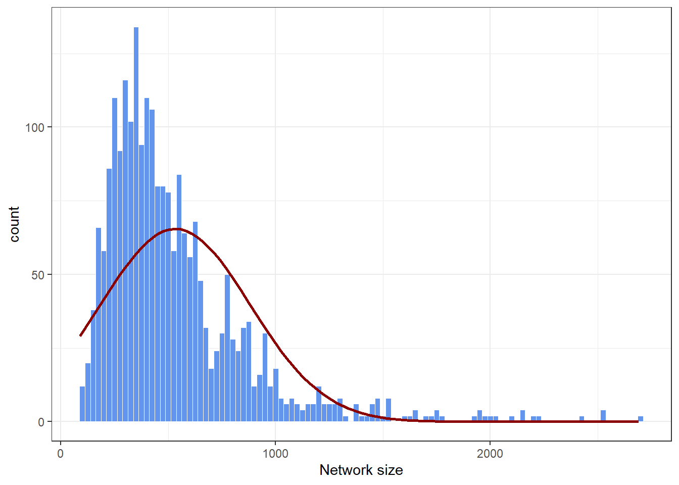

Appendix 5: Distribution of Network Size

Calculate the quantiles

quantile(df_tot$netsover3, probs = seq(0, 1, 0.2))

#>         0%        20%        40%        60%        80%       100% 
#>   89.16824  281.03725  385.51150  507.76754  730.40253 2691.24182

Use these quantiles in the regression

M3_robustness_size2 <- lmer(Y_L ~ as.factor(L_gender) + as.factor(L_groep) + as.factor(L_relatie2) +
    as.factor(L_issue) + as.factor(L_positie2) + as.factor(L_groep) + female + egoM + egoT + gen_sim +
    ethnic_sim + cage + educM + educH + (netsover3 <= quantile(df_tot$netsover3, probs = seq(0, 1, 0.2))[2]) +
    (netsover3 > quantile(df_tot$netsover3, probs = seq(0, 1, 0.2))[2] & netsover3 <= quantile(df_tot$netsover3,
        probs = seq(0, 1, 0.2))[3]) + (netsover3 > quantile(df_tot$netsover3, probs = seq(0, 1, 0.2))[3] &
    netsover3 <= quantile(df_tot$netsover3, probs = seq(0, 1, 0.2))[4]) + (netsover3 > quantile(df_tot$netsover3,
    probs = seq(0, 1, 0.2))[4] & netsover3 <= quantile(df_tot$netsover3, probs = seq(0, 1, 0.2))[5]) +
    hhi_gender + hhi_ethnic + (1 | crespnr), data = df_tot)

df <- round(as.data.frame(summary(M3_robustness_size2)$coefficients), 3) %>%
    rownames_to_column(" ")
flextable(df)

Size in quantiles
	Estimate	Std. Error	t value
(Intercept)	3.519	0.159	22.128
as.factor(L_gender)2	-0.001	0.030	-0.049
as.factor(L_groep)1	-0.059	0.040	-1.495
as.factor(L_groep)3	-0.049	0.039	-1.254
as.factor(L_relatie2)weak	-0.071	0.030	-2.350
as.factor(L_issue)2	-0.033	0.036	-0.911
as.factor(L_issue)3	0.010	0.036	0.282
as.factor(L_positie2)same	0.015	0.032	0.474
female	-0.253	0.052	-4.821
egoM	-0.008	0.086	-0.088
egoT	-0.130	0.073	-1.790
gen_sim	0.047	0.030	1.584
ethnic_sim	0.029	0.035	0.823
cage	0.000	0.003	-0.089
educM	0.301	0.080	3.744
educH	0.530	0.082	6.495
netsover3 <= quantile(df_tot$netsover3, probs = seq(0, 1, 0.2))[2]TRUE	0.018	0.091	0.204
netsover3 > quantile(df_tot$netsover3, probs = seq(0, 1, 0.2))[2] & netsover3 <= quantile(df_tot$netsover3, probs = seq(0, 1, 0.2))[3]TRUE	0.144	0.083	1.733
netsover3 > quantile(df_tot$netsover3, probs = seq(0, 1, 0.2))[3] & netsover3 <= quantile(df_tot$netsover3, probs = seq(0, 1, 0.2))[4]TRUE	0.089	0.082	1.078
netsover3 > quantile(df_tot$netsover3, probs = seq(0, 1, 0.2))[4] & netsover3 <= quantile(df_tot$netsover3, probs = seq(0, 1, 0.2))[5]TRUE	0.102	0.082	1.248
hhi_gender	0.143	0.209	0.688
hhi_ethnic	0.358	0.140	2.555

Is this consistent across ethnic groups

M3_robustness_size2 <- lmer(Y_L ~ as.factor(L_gender) + as.factor(L_groep) + as.factor(L_relatie2) +
    as.factor(L_issue) + as.factor(L_positie2) + as.factor(L_groep) + female + gen_sim + ethnic_sim +
    cage + educM + educH + (netsover3 <= quantile(df_tot$netsover3, probs = seq(0, 1, 0.2))[2]) + (netsover3 >
    quantile(df_tot$netsover3, probs = seq(0, 1, 0.2))[2] & netsover3 <= quantile(df_tot$netsover3, probs = seq(0,
    1, 0.2))[3]) + (netsover3 > quantile(df_tot$netsover3, probs = seq(0, 1, 0.2))[3] & netsover3 <=
    quantile(df_tot$netsover3, probs = seq(0, 1, 0.2))[4]) + (netsover3 > quantile(df_tot$netsover3,
    probs = seq(0, 1, 0.2))[4] & netsover3 <= quantile(df_tot$netsover3, probs = seq(0, 1, 0.2))[5]) +
    hhi_gender + hhi_ethnic + (1 | crespnr), data = df_tot[df_tot$egoNL == 1, ])

df <- round(as.data.frame(summary(M3_robustness_size2)$coefficients), 3) %>%
    rownames_to_column(" ")
flextable(df)

Size in quantiles (native Dutch only)
	Estimate	Std. Error	t value
(Intercept)	3.634	0.190	19.112
as.factor(L_gender)2	-0.003	0.038	-0.074
as.factor(L_groep)1	-0.087	0.045	-1.953
as.factor(L_groep)3	-0.046	0.046	-1.020
as.factor(L_relatie2)weak	-0.116	0.038	-3.074
as.factor(L_issue)2	-0.025	0.046	-0.540
as.factor(L_issue)3	0.012	0.044	0.277
as.factor(L_positie2)same	0.013	0.040	0.315
female	-0.338	0.064	-5.320
gen_sim	0.028	0.038	0.752
cage	0.001	0.004	0.330
educM	0.309	0.107	2.876
educH	0.478	0.110	4.350
netsover3 <= quantile(df_tot$netsover3, probs = seq(0, 1, 0.2))[2]TRUE	0.030	0.112	0.268
netsover3 > quantile(df_tot$netsover3, probs = seq(0, 1, 0.2))[2] & netsover3 <= quantile(df_tot$netsover3, probs = seq(0, 1, 0.2))[3]TRUE	0.136	0.101	1.337
netsover3 > quantile(df_tot$netsover3, probs = seq(0, 1, 0.2))[3] & netsover3 <= quantile(df_tot$netsover3, probs = seq(0, 1, 0.2))[4]TRUE	0.125	0.099	1.264
netsover3 > quantile(df_tot$netsover3, probs = seq(0, 1, 0.2))[4] & netsover3 <= quantile(df_tot$netsover3, probs = seq(0, 1, 0.2))[5]TRUE	0.039	0.097	0.398
hhi_gender	-0.067	0.252	-0.267
hhi_ethnic	0.586	0.165	3.552

M3_robustness_size2 <- lmer(Y_L ~ as.factor(L_gender) + as.factor(L_groep) + as.factor(L_relatie2) +
    as.factor(L_issue) + as.factor(L_positie2) + as.factor(L_groep) + female + gen_sim + ethnic_sim +
    cage + educM + educH + (netsover3 <= quantile(df_tot$netsover3, probs = seq(0, 1, 0.2))[2]) + (netsover3 >
    quantile(df_tot$netsover3, probs = seq(0, 1, 0.2))[2] & netsover3 <= quantile(df_tot$netsover3, probs = seq(0,
    1, 0.2))[3]) + (netsover3 > quantile(df_tot$netsover3, probs = seq(0, 1, 0.2))[3] & netsover3 <=
    quantile(df_tot$netsover3, probs = seq(0, 1, 0.2))[4]) + (netsover3 > quantile(df_tot$netsover3,
    probs = seq(0, 1, 0.2))[4] & netsover3 <= quantile(df_tot$netsover3, probs = seq(0, 1, 0.2))[5]) +
    hhi_gender + hhi_ethnic + (1 | crespnr), data = df_tot[df_tot$egoM == 1, ])

df <- round(as.data.frame(summary(M3_robustness_size2)$coefficients), 3) %>%
    rownames_to_column(" ")
flextable(df)

Size in quantiles (Moroccan Dutch only)
	Estimate	Std. Error	t value
(Intercept)	3.147	0.581	5.418
as.factor(L_gender)2	-0.047	0.087	-0.541
as.factor(L_groep)1	-0.305	0.761	-0.400
as.factor(L_groep)3	-0.127	0.107	-1.179
as.factor(L_relatie2)weak	0.007	0.084	0.088
as.factor(L_issue)2	-0.133	0.099	-1.336
as.factor(L_issue)3	-0.103	0.106	-0.974
as.factor(L_positie2)same	0.056	0.091	0.619
female	0.059	0.186	0.319
gen_sim	0.193	0.087	2.217
ethnic_sim	0.332	0.760	0.437
cage	0.009	0.009	1.041
educM	-0.034	0.210	-0.163
educH	0.329	0.228	1.440
netsover3 <= quantile(df_tot$netsover3, probs = seq(0, 1, 0.2))[2]TRUE	0.015	0.330	0.046
netsover3 > quantile(df_tot$netsover3, probs = seq(0, 1, 0.2))[2] & netsover3 <= quantile(df_tot$netsover3, probs = seq(0, 1, 0.2))[3]TRUE	0.222	0.261	0.853
netsover3 > quantile(df_tot$netsover3, probs = seq(0, 1, 0.2))[3] & netsover3 <= quantile(df_tot$netsover3, probs = seq(0, 1, 0.2))[4]TRUE	0.092	0.248	0.372
netsover3 > quantile(df_tot$netsover3, probs = seq(0, 1, 0.2))[4] & netsover3 <= quantile(df_tot$netsover3, probs = seq(0, 1, 0.2))[5]TRUE	0.232	0.254	0.913
hhi_gender	0.167	0.828	0.201
hhi_ethnic	0.389	0.614	0.633

M3_robustness_size2 <- lmer(Y_L ~ as.factor(L_gender) + as.factor(L_groep) + as.factor(L_relatie2) +
    as.factor(L_issue) + as.factor(L_positie2) + as.factor(L_groep) + female + gen_sim + ethnic_sim +
    cage + educM + educH + (netsover3 <= quantile(df_tot$netsover3, probs = seq(0, 1, 0.2))[2]) + (netsover3 >
    quantile(df_tot$netsover3, probs = seq(0, 1, 0.2))[2] & netsover3 <= quantile(df_tot$netsover3, probs = seq(0,
    1, 0.2))[3]) + (netsover3 > quantile(df_tot$netsover3, probs = seq(0, 1, 0.2))[3] & netsover3 <=
    quantile(df_tot$netsover3, probs = seq(0, 1, 0.2))[4]) + (netsover3 > quantile(df_tot$netsover3,
    probs = seq(0, 1, 0.2))[4] & netsover3 <= quantile(df_tot$netsover3, probs = seq(0, 1, 0.2))[5]) +
    hhi_gender + hhi_ethnic + (1 | crespnr), data = df_tot[df_tot$egoT == 1, ])

df <- round(as.data.frame(summary(M3_robustness_size2)$coefficients), 3) %>%
    rownames_to_column(" ")
flextable(df)

Size in quantiles (Turkish Dutch only)
	Estimate	Std. Error	t value
(Intercept)	3.568	0.368	9.688
as.factor(L_gender)2	0.042	0.061	0.691
as.factor(L_groep)1	-0.054	0.074	-0.732
as.factor(L_groep)3	-0.358	0.720	-0.497
as.factor(L_relatie2)weak	-0.016	0.064	-0.253
as.factor(L_issue)2	-0.002	0.075	-0.025
as.factor(L_issue)3	0.046	0.078	0.587
as.factor(L_positie2)same	-0.035	0.066	-0.529
female	-0.242	0.107	-2.251
gen_sim	0.028	0.061	0.457
ethnic_sim	0.333	0.719	0.464
cage	-0.007	0.006	-1.109
educM	0.467	0.161	2.912
educH	0.718	0.156	4.604
netsover3 <= quantile(df_tot$netsover3, probs = seq(0, 1, 0.2))[2]TRUE	-0.105	0.179	-0.587
netsover3 > quantile(df_tot$netsover3, probs = seq(0, 1, 0.2))[2] & netsover3 <= quantile(df_tot$netsover3, probs = seq(0, 1, 0.2))[3]TRUE	0.111	0.173	0.643
netsover3 > quantile(df_tot$netsover3, probs = seq(0, 1, 0.2))[3] & netsover3 <= quantile(df_tot$netsover3, probs = seq(0, 1, 0.2))[4]TRUE	0.042	0.184	0.230
netsover3 > quantile(df_tot$netsover3, probs = seq(0, 1, 0.2))[4] & netsover3 <= quantile(df_tot$netsover3, probs = seq(0, 1, 0.2))[5]TRUE	0.089	0.188	0.475
hhi_gender	0.642	0.403	1.596
hhi_ethnic	-0.289	0.291	-0.990

8.7.4.3 change refs cats to quantiles 2,3 and 4.

M3_robustness_size3 <- lmer(Y_L ~ as.factor(L_gender) + as.factor(L_groep) + as.factor(L_relatie2) +
    as.factor(L_issue) + as.factor(L_positie2) + as.factor(L_groep) + female + egoM + egoT + gen_sim +
    ethnic_sim + cage + educM + educH + (netsover3 <= quantile(df_tot$netsover3, probs = seq(0, 1, 0.2))[2]) +
    (netsover3 > quantile(df_tot$netsover3, probs = seq(0, 1, 0.2))[5]) + hhi_gender + hhi_ethnic + (1 |
    crespnr), data = df_tot)

df <- round(as.data.frame(summary(M3_robustness_size3)$coefficients), 3) %>%
    rownames_to_column(" ")
flextable(df)

Size in quantiles (changed ref. cat.)
	Estimate	Std. Error	t value
(Intercept)	3.633	0.148	24.536
as.factor(L_gender)2	-0.002	0.030	-0.051
as.factor(L_groep)1	-0.059	0.040	-1.492
as.factor(L_groep)3	-0.049	0.039	-1.256
as.factor(L_relatie2)weak	-0.071	0.030	-2.364
as.factor(L_issue)2	-0.033	0.036	-0.917
as.factor(L_issue)3	0.010	0.036	0.283
as.factor(L_positie2)same	0.015	0.032	0.488
female	-0.253	0.052	-4.824
egoM	-0.007	0.085	-0.078
egoT	-0.127	0.072	-1.756
gen_sim	0.048	0.030	1.599
ethnic_sim	0.030	0.035	0.838
cage	0.000	0.003	-0.067
educM	0.303	0.080	3.766
educH	0.532	0.081	6.528
netsover3 <= quantile(df_tot$netsover3, probs = seq(0, 1, 0.2))[2]TRUE	-0.096	0.072	-1.318
netsover3 > quantile(df_tot$netsover3, probs = seq(0, 1, 0.2))[5]TRUE	-0.111	0.067	-1.643
hhi_gender	0.130	0.207	0.627
hhi_ethnic	0.355	0.140	2.545

Bates, Douglas, Martin Machler, Ben Bolker, and Steve Walker. 2015. “Fitting Linear Mixed-Effects Models Using Lme4” 67. https://doi.org/10.18637/jss.v067.i01.

Jeroense, TMG, J Tolsma, M Kalmijn, GLM Kraaykamp, and Radboud University Nijmegen. 2023. “NEtherlands Longitudinal Lifecourse Study 2022 - Versie 1.0.” DANS Data Station Social Sciences; Humanities. https://doi.org/10.17026/DANS-XYK-M56B.

Long, Jacob A. 2022. Jtools: Analysis and Presentation of Social Scientific Data. https://cran.r-project.org/package=jtools.

LS0tDQp0aXRsZTogIlJFUExJQ0FUSU9OIFBBQ0tBR0U6IFRoZSBpbXBhY3Qgb2YgZHlhZHMgYW5kIGV4dGVuZGVkIG5ldHdvcmtzIG9uIHBvbGl0aWNhbCB0YWxrOiBBIGZhY3RvcmlhbCBzdXJ2ZXkgZXhwZXJpbWVudCBpbiB0aGUgTmV0aGVybGFuZHMiDQpiaWJsaW9ncmFwaHk6IHJlZmVyZW5jZXMuYmliDQotLS0gIA0KDQpgYGB7ciwgZ2xvYmFsc2V0dGluZ3MsIGVjaG89RkFMU0UsIHdhcm5pbmc9RkFMU0UsIG1lc3NhZ2U9RkFMU0UsIHJlc3VsdHM9J2hpZGUnfQ0KbGlicmFyeShrbml0cikNCm9wdHNfY2h1bmskc2V0KHRpZHkub3B0cz1saXN0KHdpZHRoLmN1dG9mZj0xMDApLHRpZHk9VFJVRSwgd2FybmluZyA9IEZBTFNFLCBtZXNzYWdlID0gRkFMU0UsY29tbWVudCA9ICIjPiIsIGNhY2hlPVRSVUUsIGNsYXNzLnNvdXJjZT1jKCJ0ZXN0IiksIGNsYXNzLm91dHB1dD1jKCJ0ZXN0MiIpLCByZXN1bHRzID0gImhvbGQiLCBjYWNoZS5sYXp5ID0gRkFMU0UpDQpvcHRpb25zKHdpZHRoID0gMTAwKSANCnJnbDo6c2V0dXBLbml0cigpDQoNCmNvbG9yaXplIDwtIGZ1bmN0aW9uKHgsIGNvbG9yKSB7c3ByaW50ZigiPHNwYW4gc3R5bGU9J2NvbG9yOiAlczsnPiVzPC9zcGFuPiIsIGNvbG9yLCB4KSB9DQoNCmBgYA0KDQpgYGB7ciBrbGlwcHksIGVjaG89RkFMU0UsIGluY2x1ZGU9VFJVRSwgbWVzc2FnZT1GQUxTRX0NCiMgaW5zdGFsbC5wYWNrYWdlcygicmVtb3RlcyIpDQojcmVtb3Rlczo6aW5zdGFsbF9naXRodWIoInJsZXN1ci9rbGlwcHkiKQ0Ka2xpcHB5OjprbGlwcHkocG9zaXRpb24gPSBjKCd0b3AnLCAncmlnaHQnKSkNCiNrbGlwcHk6OmtsaXBweShjb2xvciA9ICdkYXJrcmVkJykNCiNrbGlwcHk6OmtsaXBweSh0b29sdGlwX21lc3NhZ2UgPSAnQ2xpY2sgdG8gY29weScsIHRvb2x0aXBfc3VjY2VzcyA9ICdEb25lJykNCmBgYA0KDQoNCi0tLS0NCiAgDQojIEludHJvZHVjdGlvbiAgDQoNCg0KVGhpcyB3ZWJzaXRlIGlzIGEgc3VwcGxlbWVudCB0byB0aGUgcGFwZXIgKipUaGUgaW1wYWN0IG9mIGR5YWRzIGFuZCBleHRlbmRlZCBuZXR3b3JrcyBvbiBwb2xpdGljYWwgdGFsazogQSBmYWN0b3JpYWwgc3VydmV5IGV4cGVyaW1lbnQgaW4gdGhlIE5ldGhlcmxhbmRzKiogSXQgY29udGFpbnMgdGhlIGxpbmsgdG8gdGhlIHB1YmxpY2x5IGF2YWlsYWJsZSBkYXRhIHNldCB3ZSB1c2VkIFtORUxMU10oaHR0cHM6Ly9kb2kub3JnLzEwLjE3MDI2L0RBTlMtWFlLLU01NkIpIGFuZCBhbGwgdGhlIG5lY2Vzc2FyeSBSIGNvZGUgdG8gcmVwbGljYXRlIG91ciByZXBvcnRlZCByZXN1bHRzIGFuZCB0YWJsZXMuIA0KDQpIb2ZzdHJhLCBCLiwgSmVyb2Vuc2UsIFQuLCBUb2xzbWEsIEouICgyMDI2KS4gVGhlIGltcGFjdCBvZiBkeWFkcyBhbmQgZXh0ZW5kZWQgbmV0d29ya3Mgb24gcG9saXRpY2FsIHRhbGs6IEEgZmFjdG9yaWFsIHN1cnZleSBleHBlcmltZW50IGluIHRoZSBOZXRoZXJsYW5kcy4gKlNvY2lhbCBOZXR3b3JrcyosICo4NSosIDY2LTY3IFtwZGZdKGh0dHBzOi8vd3d3LnNjaWVuY2VkaXJlY3QuY29tL3NjaWVuY2UvYXJ0aWNsZS9waWkvUzAzNzg4NzMzMjUwMDA4MDIvcGRmZnQ/bWQ1PWVjZjNlOWUzMDdkZGY3ZDMxODg4Zjk0NDJhNzYwMzY0JnBpZD0xLXMyLjAtUzAzNzg4NzMzMjUwMDA4MDItbWFpbi5wZGYpIFtkb2ldKGh0dHBzOi8vZG9pLm9yZy8xMC4xMDE2L2ouc29jbmV0LjIwMjUuMTEuMDAzKQ0KDQojIyBDb250YWN0DQoNClF1ZXN0aW9ucyBjYW4gYmUgYWRkcmVzc2VkIHRvIFtCYXMgSG9mc3RyYV0obWFpbHRvOmJhcy5ob2ZzdHJhQHJ1Lm5sKQ0KDQojIyBnZW5lcmFsIGN1c3RvbSBmdW5jdGlvbnMNCg0KLSBgZnBhY2thZ2UuY2hlY2tgOiBDaGVjayBpZiBwYWNrYWdlcyBhcmUgaW5zdGFsbGVkIChhbmQgaW5zdGFsbCBpZiBub3QpIGluIFINCi0gYGZzYXZlYDogRnVuY3Rpb24gdG8gc2F2ZSBkYXRhIHdpdGggdGltZSBzdGFtcCBpbiBjb3JyZWN0IGRpcmVjdG9yeQ0KLSBgZmxvYWRgOiBGdW5jdGlvbiB0byBsb2FkIFItb2JqZWN0cyB1bmRlciBuZXcgbmFtZXMNCi0gYGZzaG93ZGZgOiBQcmludCBvYmplY3RzIChgdGliYmxlYCAvIGBkYXRhLmZyYW1lYCkgbmljZWx5IG9uIHNjcmVlbiBpbiBgLlJtZGANCi0gYGZ0aGVtZWA6IHByZXR0eSBnZ3Bsb3QyIHRoZW1lDQoNCmBgYHtyLCBmdW59DQpmcGFja2FnZS5jaGVjayA8LSBmdW5jdGlvbihwYWNrYWdlcykgew0KICAgIGxhcHBseShwYWNrYWdlcywgRlVOID0gZnVuY3Rpb24oeCkgew0KICAgICAgICBpZiAoIXJlcXVpcmUoeCwgY2hhcmFjdGVyLm9ubHkgPSBUUlVFKSkgew0KICAgICAgICAgICAgaW5zdGFsbC5wYWNrYWdlcyh4LCBkZXBlbmRlbmNpZXMgPSBUUlVFKQ0KICAgICAgICAgICAgbGlicmFyeSh4LCBjaGFyYWN0ZXIub25seSA9IFRSVUUpDQogICAgICAgIH0NCiAgICB9KQ0KfQ0KDQpmc2F2ZSA8LSBmdW5jdGlvbih4LCBsb2NhdGlvbiA9ICIuL2RhdGEvcHJvY2Vzc2VkLyIpIHsNCiAgaWYgKGxvY2F0aW9uID09ICIuL2RhdGEvcHJvY2Vzc2VkLyIpIHsNCiAgaWZlbHNlKCFkaXIuZXhpc3RzKCJkYXRhIiksIGRpci5jcmVhdGUoImRhdGEiKSwgRkFMU0UpDQogIGlmZWxzZSghZGlyLmV4aXN0cygiZGF0YS9wcm9jZXNzZWQiKSwgZGlyLmNyZWF0ZSgiZGF0YS9wcm9jZXNzZWQiKSwgRkFMU0UpDQogIH0NCg0KICBvYmplY3QgPSBkZXBhcnNlKHN1YnN0aXR1dGUoeCkpDQogIGRhdGVuYW1lIDwtIHN1YnN0cihnc3ViKCJbOi1dIiwgIiIsIFN5cy50aW1lKCkpLCAxLCA4KQ0KICB0b3RhbG5hbWUgPC0gcGFzdGUobG9jYXRpb24sIG9iamVjdCwgIl8iLCBkYXRlbmFtZSwgICIucmRhIiwgc2VwID0gIiIpDQogIGFzc2lnbihldmFsKG9iamVjdCksIHgsIGVudmlyID0gLkdsb2JhbEVudikNCiAgcHJpbnQocGFzdGUoIlNBVkVEOiAiLCB0b3RhbG5hbWUsIHNlcCA9ICIiKSkNCiAgc2F2ZShsaXN0ID0gb2JqZWN0LCBmaWxlID0gdG90YWxuYW1lKSAgDQp9DQoNCmZsb2FkICA8LSBmdW5jdGlvbihmaWxlTmFtZSl7DQogIGxvYWQoZmlsZU5hbWUpDQogIGdldChscygpW2xzKCkgIT0gImZpbGVOYW1lIl0pDQp9DQoNCg0KZnNob3dkZiA8LSBmdW5jdGlvbih4LCBjYXB0aW9uID0gTlVMTCwgLi4uKSB7DQogICAga25pdHI6OmthYmxlKHgsIGRpZ2l0cyA9IDIsICJodG1sIiwgY2FwdGlvbiA9IGNhcHRpb24sIC4uLikgJT4lDQogICAgICAgIGthYmxlRXh0cmE6OmthYmxlX3N0eWxpbmcoYm9vdHN0cmFwX29wdGlvbnMgPSBjKCJzdHJpcGVkIiwgImhvdmVyIikpICU+JQ0KICAgICAgICBrYWJsZUV4dHJhOjpzY3JvbGxfYm94KHdpZHRoID0gIjEwMCUiLCBoZWlnaHQgPSAiMzAwcHgiKQ0KfQ0KDQpmdGhlbWUgPC0gZnVuY3Rpb24oKSB7DQogICNkb3dubG9hZCBmb250IGF0IGh0dHBzOi8vZm9udHMuZ29vZ2xlLmNvbS9zcGVjaW1lbi9Kb3N0Lw0KICB0aGVtZV9taW5pbWFsKGJhc2VfZmFtaWx5ID0gIkpvc3QiKSArDQogICAgdGhlbWUocGFuZWwuZ3JpZC5taW5vciA9IGVsZW1lbnRfYmxhbmsoKSwNCiAgICAgICAgICBwbG90LnRpdGxlID0gZWxlbWVudF90ZXh0KGZhbWlseSA9ICJKb3N0IiwgZmFjZSA9ICJib2xkIiksDQogICAgICAgICAgYXhpcy50aXRsZSA9IGVsZW1lbnRfdGV4dChmYW1pbHkgPSAiSm9zdCBNZWRpdW0iKSwNCiAgICAgICAgICBheGlzLnRpdGxlLnggPSBlbGVtZW50X3RleHQoaGp1c3QgPSAwKSwNCiAgICAgICAgICBheGlzLnRpdGxlLnkgPSBlbGVtZW50X3RleHQoaGp1c3QgPSAxKSwNCiAgICAgICAgICBzdHJpcC50ZXh0ID0gZWxlbWVudF90ZXh0KGZhbWlseSA9ICJKb3N0IiwgZmFjZSA9ICJib2xkIiwNCiAgICAgICAgICAgICAgICAgICAgICAgICAgICAgICAgICAgIHNpemUgPSByZWwoMC43NSksIGhqdXN0ID0gMCksDQogICAgICAgICAgc3RyaXAuYmFja2dyb3VuZCA9IGVsZW1lbnRfcmVjdChmaWxsID0gImdyZXk5MCIsIGNvbG9yID0gTkEpLA0KICAgICAgICAgIGxlZ2VuZC5wb3NpdGlvbiA9ICJib3R0b20iKQ0KfQ0KYGBgDQoNCg0KDQoNCjxicj4NCg0KIyMgbmVjZXNzYXJ5IHBhY2thZ2VzDQoNClRvIGZ1cnRoZXIgZWFzZSByZXBsaWNhdGlvbiBwdXJwb3NlcyB3ZSB1c2UgZ3JvdW5kaG9nLiANCg0KDQpgYGB7ciwgcGFja2FnZXMsIG1lc3NhZ2U9RkFMU0UsIHJlc3VsdHM9J2hpZGUnLCB3YXJuaW5nPUZBTFNFfQ0KcGFja2FnZXMgPC0gYygndGlkeXZlcnNlJywgJ2xtZTQnLCAncHN5Y2gnICwnb3JkaW5hbCcsJ2dncGxvdDInLCAnb2ZmaWNlcicsICdmbGV4dGFibGUnLCAnSG1pc2MnLCAnanRvb2xzJywgJ3BhcmFsbGVsJykNCmZwYWNrYWdlLmNoZWNrKHBhY2thZ2VzKQ0KYGBgDQoNCjxicj4NCg0KIyMgc2Vzc2lvbiBpbmZvDQoNCmBgYHtyfQ0Kc2Vzc2lvbkluZm8oKQ0KYGBgDQoNCg0KYGBge3IgZm9udHMsIGVjaG89RkFMU0UsIHdhcm5pbmc9RkFMU0UsIHJlc3VsdHM9J2hpZGUnLCBldmFsPUZBTFNFfQ0KIyBpbXBvcnQgZm9udCBKT1NUDQojZXh0cmFmb250Ojpmb250X2ltcG9ydChwYXR0ZXJuID0gIkpvc3QiKQ0KI2V4dHJhZm9udDo6bG9hZGZvbnRzKGRldmljZT0id2luIikNCg0KIyBTZXQgZGVmYXVsdCB0aGVtZSBhbmQgZm9udCBzdHVmZg0KZ2dwbG90Mjo6dGhlbWVfc2V0KGZ0aGVtZSgpKQ0KZ2dwbG90Mjo6dXBkYXRlX2dlb21fZGVmYXVsdHMoInRleHQiLCBsaXN0KGZhbWlseSA9ICJKb3N0IiwgZm9udGZhY2UgPSAicGxhaW4iKSkNCmdncGxvdDI6OnVwZGF0ZV9nZW9tX2RlZmF1bHRzKCJsYWJlbCIsIGxpc3QoZmFtaWx5ID0gIkpvc3QiLCBmb250ZmFjZSA9ICJwbGFpbiIpKQ0KYGBgDQoNCg0KLS0tDQoNCiMgTkVMTFMNCg0KV2UgdXNlIHRoZSB0aGlyZCB3YXZlIG9mIHRoZSBORXRoZXJsYW5kcyBMb25naXR1ZGluYWwgTGlmZWNvdXJzZSBTdHVkeSBbQGplcm9lbnNlMjAyM10uIFRoaXMgZGF0YXNldCBpcyBwdWJsaWNhbGx5IGF2YWlsYWJsZSBhdCBEQU5TIERhdGEgU3RhdGlvbiBTb2NpYWwgU2NpZW5jZXMgYW5kIEh1bWFuaXRpZXMsIHNlZSBbaHR0cHM6Ly9kb2kub3JnLzEwLjE3MDI2L0RBTlMtWFlLLU01NkJdKGh0dHBzOi8vZG9pLm9yZy8xMC4xNzAyNi9EQU5TLVhZSy1NNTZCKS4gUGxlYXNlIG1ha2Ugc3VyZSB0byBkb3dubG9hZCB0aGUgZGF0YXNldCB3aXRoIHRoZSB2YXJpYWJsZXMgdGhhdCB3ZXJlIG9yaWdpbmFsbHkgdW5kZXIgZW1iYXJnbyBpbmNsdWRlZC4gDQoNCmBgYHtyfQ0KI2RmIDwtIGZsb2FkKCJEYXRhLzIwMjMtMDQtMDZfbmVsbHMtY2xlYW5lZC0yMi1WMS4wLlJkYXRhIikNCmRmX2RhbnMgPC0gZmxvYWQoIkRhdGEvbmVsbHMtMjJfVjEuMS5SZGF0YSIpDQpkZiA8LSBkZl9kYW5zDQpgYGANCg0KDQojIyBnZW5kZXIgYW5kIGV0aG5pYyBiYWNrZ3JvdW5kDQoNCmBgYHtyfQ0KZGYkZmVtYWxlIDwtIGFzLm51bWVyaWMoZGYkQjAyPT0yKSAjZ2VuZGVyDQoNCiNldG5pY2l0eSwgbm8gbWlzc2luZ3MNCmRmJGVnb05MIDwtIGFzLm51bWVyaWMoZGYkQjA1ID09IDEgJiBkZiRCMDYgPT0gMSAmIGRmJEIwNyA9PSAxKQ0KZGYkZWdvTSA8LSBhcy5udW1lcmljKGRmJEIwNSA9PSAyIHwgZGYkQjA2ID09IDIgfCBkZiRCMDcgPT0gMikNCmRmJGVnb1QgPC0gYXMubnVtZXJpYyhkZiRCMDUgPT0gMyB8IGRmJEIwNiA9PSAzIHwgZGYkQjA3ID09IDMpDQpkZiRlZ29NIDwtIGlmZWxzZShkZiRCMDYgPT0gMiwgMSwgZGYkZWdvTSkgI21vdGhlciBkb21pbmFudA0KZGYkZWdvVCA8LSBpZmVsc2UoZGYkQjA2ID09IDMsIDEsIGRmJGVnb1QpICNtb3RoZXIgZG9taW5hbnQNCmRmJGVnb08gPC0gYXMubnVtZXJpYyhkZiRlZ29OTCAhPSAxICYgZGYkZWdvTSAhPSAxICYgZGYkZWdvVCAhPSAxKSAjb3RoZXIsIG5lZWQgdG8gZmlsdGVyDQojZ2VuZXJhdGlvbg0KZGYkZWdvX2dlbjEgPC0gYXMubnVtZXJpYyhkZiRCMDUgPT0gMiB8IGRmJEIwNSA9PSAzICkNCg0KIyB0YWJsZShkZiRlZ29NLCB1c2VOQSA9ICJhbHdheXMiKSANCiMgdGFibGUoZGYkZWdvVCwgdXNlTkEgPSAiYWx3YXlzIikgDQojIHRhYmxlKGRmJGVnb08sIHVzZU5BID0gImFsd2F5cyIpICNuZWVkIHRvIGZpbHRlcg0KYGBgDQoNCiMjIGFnZSBhbmQgZWR1Y2F0aW9uIA0KDQpgYGB7cn0NCiNhZ2UNCiN0YWJsZShpcy5uYShkZiRjYWdlKSkNCg0KI2VkdWNhdGlvbg0KZGYkZWR1Y0wgPC0gYXMubnVtZXJpYyhkZiRDMDUgPCA1IHwgZGYkQzA1ID09IDEzICkgIyBsb3dlciB0aGFuIEhhdm8NCmRmJGVkdWNNIDwtIGFzLm51bWVyaWMoKGRmJEMwNSA+IDQgJiBkZiRDMDUgPCA5KSB8IGRmJEMwNSA9PSAxNCApICMgaGF2ZSwgdndvLCBtYm8NCmRmJGVkdWNIIDwtIGFzLm51bWVyaWMoKGRmJEMwNSA+IDggJiBkZiRDMDUgPCAxMykgfCBkZiRDMDUgPT0gMTUgKSAjIGhibywgd28NCmRmJGVkdWNfY3VycmVudCA8LSBhcy5udW1lcmljKGRmJEMwMyA9PSAxKSAjIGN1cnJlbnRseSBmdWxsLXRpbWUgaW4gZWR1Yw0KDQpgYGANCg0KDQojIyBhZGRpdGlvbmFsIHBvdGVudGlhbCBjb250cm9scyANCg0KYGBge3IsIHJlc3VsdHM9J2hpZGUnfQ0KI3BvbGl0aWNhbCBvcGluaW9ucw0KI0gxMmQuIERlIG92ZXJoZWlkIG1vZXQgZGUgaW5rb21lbnN2ZXJzY2hpbGxlbiBpbiBOZWRlcmxhbmQga2xlaW5lciBtYWtlbg0KI0gxMmUuIERlIHRvcGlua29tZW5zIGluIGhldCBiZWRyaWpmc2xldmVuIHppam4gdGUgaG9vZw0KI0gxMmYuIERlIG92ZXJoZWlkIG1vZXQgZGUgc29jaWFsZSB1aXRrZXJpbmdlbiB2ZXJob2dlbg0KI2F0dHJpYnV0ZXMoZGYkSDEyZSkNCg0KZGYkZWdvX29waW5pb24xIDwtIGRmJEgxMmUNCmRmJGVnb19vcGluaW9uMWIgPC0gcm93TWVhbnMoY2JpbmQoZGYkSDEyZCwgZGYkSDEyZSwgZGYkSDEyZiksIG5hLnJtID0gVCkNCiN0YWJsZShkZiRlZ29fb3BpbmlvbjEsIHVzZU5BID0gImFsd2F5cyIpDQoNCiNIMTJhLiBBbHMgZWVuIGxhbmQgc3Bhbm5pbmdlbiB3aWwgdmVybWluZGVyZW4gbW9ldCBkZSBpbW1pZ3JhdGllIHN0b3BwZW4NCmRmJGVnb19vcGluaW9uMiA8LSBkZiRIMTJhDQojYXR0cmlidXRlcyhkZiRIMTJhKQ0KI3JldmVyc2UgY29kaW5nDQpkZiRlZ29fb3BpbmlvbjIgPC0gNiAtIGRmJGVnb19vcGluaW9uMg0KDQojSDEzZC4gSGV0IGtsaW1hYXQgdmVyYmV0ZXJlbiBtb2V0IHByaW9yaXRlaXQgaGViYmVuLCB6ZWxmcyBhbHMgZGl0IGRlIGVjb25vbWlzY2hlIGdyb2VpIHZlcnRyYWFndA0KZGYkZWdvX29waW5pb24zIDwtIGRmJEgxM2QNCiMgdGFibGUoZGYkZWdvX29waW5pb24zLCB1c2VOQSA9ICJhbHdheXMiKQ0KI2F0dHJpYnV0ZXMoZGYkSDEzZCkNCg0KZGYgJT4lIHNlbGVjdChjKGVnb19vcGluaW9uMSwgZWdvX29waW5pb24yLCBlZ29fb3BpbmlvbjMsIGVnb19vcGluaW9uMWIsIEgxMmQsIEgxMmUsIEgxMmYpKSAlPiUgDQogIGFzLm1hdHJpeCgpICU+JQ0KICBIbWlzYzo6cmNvcnIoKQ0KDQojZmVlbGluZyB0aGVybW9tZXRlcnMgDQpkZiR0aGVybW9EIDwtIGRmJEgxOWkgDQpkZiR0aGVybW9NIDwtIGRmJEgxOWoNCmRmJHRoZXJtb1QgPC0gZGYkSDE5ayANCg0KIyBIMDYuIFBvbGl0aWNhbCBpbnRlcmVzdA0KZGYkcG9saW50IDwtIGRmJEgwNg0KIyB0YWJsZShkZiRIMDYsIHVzZU5BID0gImFsd2F5cyIpDQojYXR0cmlidXRlcyhkZiRIMDYpDQoNCiNkaXN0cmljdCB2YXJpYWJsZXM6IGdlbmRlciBhbmQgZXRobmljIGRpdmVyc2l0eQ0KZGYgPC0gZGYgJT4lDQogIG11dGF0ZShjZGlzdHJpY3QyMDIwX2FfbmwgPSBjZGlzdHJpY3QyMDIwX2FfaW53IC0gY2Rpc3RyaWN0MjAyMF9hX3dfYWxsIC0gY2Rpc3RyaWN0MjAyMF9hX3dfYWxsLCANCiAgICAgICAgIGRpc3RyaWN0X0VJX2V0aG5pYyA9IGNhc2Vfd2hlbihlZ29OTCA9PSAxIH4gKGNkaXN0cmljdDIwMjBfYV9ubCAtIChjZGlzdHJpY3QyMDIwX2FfaW53IC0gY2Rpc3RyaWN0MjAyMF9hX25sKSkgLyBjZGlzdHJpY3QyMDIwX2FfaW53LA0KICAgICAgICAgICAgICAgICAgICAgICAgICAgICAgIGVnb00gPT0gMSB+IChjZGlzdHJpY3QyMDIwX2FfbWFyb2sgLSAoY2Rpc3RyaWN0MjAyMF9hX2ludyAtIGNkaXN0cmljdDIwMjBfYV9tYXJvaykpIC8gY2Rpc3RyaWN0MjAyMF9hX2ludywNCiAgICAgICAgICAgICAgICAgICAgICAgICAgICAgICBlZ29UID09IDEgfiAoY2Rpc3RyaWN0MjAyMF9hX3R1ciAtIChjZGlzdHJpY3QyMDIwX2FfaW53IC0gY2Rpc3RyaWN0MjAyMF9hX3R1cikpIC8gY2Rpc3RyaWN0MjAyMF9hX2ludywNCiAgICAgICAgICAgICAgICAgICAgICAgIC5kZWZhdWx0ID0gTkEgKSwNCiAgICAgICAgIGRpc3RyaWN0X0VJX2dlbmRlciA9IGNhc2Vfd2hlbihmZW1hbGUgPT0gMSB+IChjZGlzdHJpY3QyMDIwX2FfdnJvdXcgLSBjZGlzdHJpY3QyMDIwX2FfbWFuKSAvIChjZGlzdHJpY3QyMDIwX2FfdnJvdXcgKyBjZGlzdHJpY3QyMDIwX2FfbWFuKSwNCiAgICAgICAgICAgICAgICAgICAgICAgICAgICAgICBmZW1hbGUgPT0gMCB+IChjZGlzdHJpY3QyMDIwX2FfbWFuIC0gY2Rpc3RyaWN0MjAyMF9hX3Zyb3V3KSAvIChjZGlzdHJpY3QyMDIwX2FfdnJvdXcgKyBjZGlzdHJpY3QyMDIwX2FfbWFuKSkpICU+JSANCiAgICBtdXRhdGUoDQogICAgZGlzdHJpY3RfRUlfZXRobmljID0gaWZlbHNlKGRpc3RyaWN0X0VJX2V0aG5pYyA+IDEgfCBkaXN0cmljdF9FSV9ldGhuaWMgPCAtMSAsIE5BLCBkaXN0cmljdF9FSV9ldGhuaWMpLA0KICAgIGRpc3RyaWN0X0VJX2dlbmRlciA9IGlmZWxzZShkaXN0cmljdF9FSV9nZW5kZXIgPiAxIHwgZGlzdHJpY3RfRUlfZ2VuZGVyIDwgLTEgLCBOQSwgZGlzdHJpY3RfRUlfZ2VuZGVyKSkNCg0KI0NvcmUgRGlzY3Vzc2lvbiBOZXR3b3JrIChzaXplIG9mIG5vbi1raW4gbmV0d29yaywgZ2VuZGVyL2V0aG5pYyBFSSApDQpkZiA8LSBkZiAlPiUNCiAgbXV0YXRlKA0KICAgIGFjcm9zcyhJMDJhOkkwNWUsIH5yZXBsYWNlX25hKC54LCAtMSkpICNyZXBsYWNlIE5BJ3Mgd2l0aCAtMQ0KICApICU+JQ0KICBtdXRhdGUoDQogICAgY2RuX3RvdCA9IDUgLSByb3dTdW1zKGNiaW5kKGlzLm5hKGRmJGNhbHRlcl9pZDEpICxpcy5uYShkZiRjYWx0ZXJfaWQyKSxpcy5uYShkZiRjYWx0ZXJfaWQzKSxpcy5uYShkZiRjYWx0ZXJfaWQ0KSwgaXMubmEoZGYkY2FsdGVyX2lkNSkgKSkpICU+JQ0KICAgIHJvd3dpc2UoKSAlPiUgIA0KICAjdG8gYmUgYWJsZSB0byBjb3VudCB2YWx1ZXMgYWNyb3NzIHZhcmlhYmxlcyBmb3IgZWFjaCByb3cNCiAgICBtdXRhdGUoDQogICAgbmthID0gIShJMDJhPDQgJiBJMDJhID4gMSksIA0KICAgIG5rYiA9ICEoSTAyYjw0ICYgSTAyYiA+IDEpLA0KICAgIG5rYyA9ICEoSTAyYzw0ICYgSTAyYyA+IDEpLA0KICAgIG5rZCA9ICEoSTAyZDw0ICYgSTAyZCA+IDEpLA0KICAgIG5rZSA9ICEoSTAyZTw0ICYgSTAyZSA+IDEpLA0KICAgIGNkbl90b3RfbmsgPSBjZG5fdG90IC0gIHN1bShjKEkwMmE8NCAmIEkwMmEgPiAxICxJMDJiPDQgJiBJMDJiID4gMSAsSTAyYzw0ICYgSTAyYyA+IDEsSTAyZDw0ICYgSTAyZCA+IDEsSTAyZTw0ICYgSTAyZSA+IDEpKSwgDQogICAgY2RuX05MID0gc3VtKGMobmthICYgSTA0YSA9PSAxICxua2IgJiBJMDRiID09IDEsbmtjICYgSTA0YyA9PSAxLCBua2QgJiBJMDRkID09IDEsIG5rZSAmIEkwNGUgPT0gMSApKSwNCiAgICBjZG5fTSA9IHN1bShjKG5rYSAmIEkwNGEgPT0gMiAsbmtiICYgSTA0YiA9PSAyLG5rYyAmIEkwNGMgPT0gMiwgbmtkICYgSTA0ZCA9PSAyLCBua2UgJiBJMDRlID09IDIgKSksDQogICAgY2RuX1QgPSBzdW0oYyhua2EgJiBJMDRhID09IDMgLG5rYiAmIEkwNGIgPT0gMyxua2MgJiBJMDRjID09IDMsIG5rZCAmIEkwNGQgPT0gMywgbmtlICYgSTA0ZSA9PSAzICkpLA0KICAgIGNkbl9PID0gc3VtKGMobmthICYgSTA0YSA9PSA0ICxua2IgJiBJMDRiID09IDQsbmtjICYgSTA0YyA9PSA0LCBua2QgJiBJMDRkID09IDQsIG5rZSAmIEkwNGUgPT0gNCApKSwNCiAgICBjZG5fbWVuID0gc3VtKGMobmthICYgSTAzYSA9PSAxICxua2IgJiBJMDNiID09IDEsbmtjICYgSTAzYyA9PSAxLCBua2QgJiBJMDNkID09IDEsIG5rZSAmIEkwM2UgPT0gMSApKSwNCiAgICBjZG5fd29tZW4gPSBzdW0oYyhua2EgJiBJMDNhID09IDIgLG5rYiAmIEkwM2IgPT0gMixua2MgJiBJMDNjID09IDIsIG5rZCAmIEkwM2QgPT0gMiwgbmtlICYgSTAzZSA9PSAyICkpDQogICkgJT4lDQogIHVuZ3JvdXAoKSAlPiUgDQogICNoaWdoZXIgRUkgc2NvcmVzIGluZGljYXRlIG1vcmUgaW50cmFncm91cCB0aWVzIHRoYW4gaW50ZXJncm91cCB0aWVzLiByYW5nZSAtMSB0byAxLCBub3RlIG9ubHkgcmVsdmFudCBpZiBzaXplPjANCiAgbXV0YXRlKGNkbl9FSV9ldGhuaWMgPSBjYXNlX3doZW4oZWdvTkwgPT0gMSB+IChjZG5fTkwgLSAoY2RuX3RvdF9uayAtIGNkbl9OTCkpIC8gY2RuX3RvdF9uaywNCiAgICAgICAgICAgICAgICAgICAgICAgICAgICAgICBlZ29NID09IDEgfiAoY2RuX00gLSAoY2RuX3RvdF9uayAtIGNkbl9NKSkgLyBjZG5fdG90X25rLA0KICAgICAgICAgICAgICAgICAgICAgICAgICAgICAgIGVnb1QgPT0gMSB+IChjZG5fVCAtIChjZG5fdG90X25rIC0gY2RuX1QpKSAvIGNkbl90b3RfbmssDQogICAgICAgICAgICAgICAgICAgICAgICAuZGVmYXVsdCA9IE5BICksDQogICAgICAgICBjZG5fRUlfZ2VuZGVyID0gY2FzZV93aGVuKGZlbWFsZSA9PSAxIH4gKGNkbl93b21lbiAtIChjZG5fdG90X25rIC0gY2RuX3dvbWVuKSkgLyBjZG5fdG90X25rLA0KICAgICAgICAgICAgICAgICAgICAgICAgICAgICAgIGZlbWFsZSA9PSAwIH4gKGNkbl9tZW4gLSAoY2RuX3RvdF9uayAtIGNkbl9tZW4pKSAvIGNkbl90b3RfbmssDQogICAgICAgICAgICAgICAgICAgICAgICAuZGVmYXVsdCA9IE5BICkpICU+JSANCiAgbXV0YXRlKGFjcm9zcyhjKGNkbl90b3Q6Y2RuX0VJX2dlbmRlciksIH4gaWZlbHNlKGlzLm5hKEgxOW8pICYgaXMubmEoSjAxYSksIE5BLCAuKSkpICU+JSANCiAgI2lmIHJlc3BvbmRlbnRzIGRpZCBub3QgYW5zd2VyIHF1ZXN0aW9ucywgcmVwbGFjZSB2YWx1ZXMgd2l0aCBOQQ0KICBtdXRhdGUoDQogICAgY2RuX0VJX2V0aG5pYyA9IGlmZWxzZShjZG5fRUlfZXRobmljID4gMSB8IGNkbl9FSV9ldGhuaWMgPCAtMSAsIE5BLCBjZG5fRUlfZXRobmljKSwNCiAgICBjZG5fRUlfZ2VuZGVyID0gaWZlbHNlKGNkbl9FSV9nZW5kZXIgPiAxIHwgY2RuX0VJX2dlbmRlciA8IC0xICwgTkEsIGNkbl9FSV9nZW5kZXIpDQogICkgDQojZmV3IGRhdGEgZGlzY3JlcGFuY2llcyANCiN0YWJsZShkZiRjZG5fRUlfZXRobmljKQ0KYGBgDQoNCiMjIE5TVU0gDQoNCkZvciBjb25zdHJ1Y3Rpb24gc2VlIFtoZXJlXSguL25zdW1fbWV0cmljcy5odG1sKS4gDQoNCmBgYHtyfQ0KbnN1bSA8LSBmbG9hZCgiLi9EYXRhL25zdW1fb3V0Y29tZXMvbnN1bV9zaXplX2RpdmVyc2l0eS5yZGEiKQ0KYGBgDQoNCiMjIyBkaXZlcnNpdHkgbWVhc3VyZXMNCg0KSGlnaGVyIHNjb3JlcyBtb3JlIGRpdmVyc2l0eS4gDQpgYGB7cn0NCm5zdW0kaGhpX2V0aG5pYyA8LSAxIC0gbnN1bSRoaGlfZXRobmljDQpuc3VtJGhoaV9nZW5kZXIgPC0gMSAtIG5zdW0kaGhpX2dlbmRlcg0KbnN1bSRoaGlfZWR1YyA8LSAxIC0gbnN1bSRoaGlfZWR1Yw0KYGBgDQoNCmBgYHtyfQ0KZGYgPC0gZGYgJT4lDQogIGxlZnRfam9pbih5PW5zdW0pIA0KDQojY2FsY3VsYXRlIHRoZSBFSSBzY29yZXMNCmRmIDwtIGRmICU+JSANCiAgbXV0YXRlKA0KICAgIG5zdW1fRUlfZXRobmljID0gY2FzZV93aGVuKA0KICAgICAgZWdvTkwgPT0gMSB+IChuc3VtX2R1dCAtIChuc3VtX21vciArIG5zdW1fdHVyKSkgLyAobnN1bV9kdXQgKyBuc3VtX21vciArIG5zdW1fdHVyKSAsDQogICAgICBlZ29NID09IDEgfiAobnN1bV9tb3IgLSAobnN1bV9kdXQgKyBuc3VtX3R1cikpIC8gKG5zdW1fZHV0ICsgbnN1bV9tb3IgKyBuc3VtX3R1ciksDQogICAgICBlZ29UID09IDEgfiAobnN1bV90dXIgLSAobnN1bV9kdXQgKyBuc3VtX21vcikpIC8gKG5zdW1fZHV0ICsgbnN1bV9tb3IgKyBuc3VtX3R1ciksDQogICAgICAgICAgICAgICAgICAgICAgICAuZGVmYXVsdCA9IE5BICksDQogICAgbnN1bV9FSV9nZW5kZXIgPSBjYXNlX3doZW4oDQogICAgICBmZW1hbGUgPT0gMSB+IChuc3VtX3dvbWVuIC0gKG5zdW1fbWVuKSkgLyAobnN1bV93b21lbiArIG5zdW1fbWVuKSwNCiAgICAgIGZlbWFsZSA9PSAwIH4gKG5zdW1fbWVuIC0gKG5zdW1fd29tZW4pKSAvIChuc3VtX3dvbWVuICsgbnN1bV9tZW4pLA0KICAgICAgICAgICAgICAgICAgICAgICAgLmRlZmF1bHQgPSBOQSApKSAlPiUgDQogIG11dGF0ZSgNCiAgICBuc3VtX0VJX2V0aG5pYyA9IGlmZWxzZShuc3VtX0VJX2V0aG5pYyA+IDEgfCBuc3VtX0VJX2V0aG5pYyA8IC0xICwgTkEsIG5zdW1fRUlfZXRobmljKSwNCiAgICBuc3VtX0VJX2dlbmRlciA9IGlmZWxzZShuc3VtX0VJX2dlbmRlciA+IDEgfCBuc3VtX0VJX2dlbmRlciA8IC0xICwgTkEsIG5zdW1fRUlfZ2VuZGVyKSkNCg0KYGBgDQoNCmBgYHtyLCBlY2hvPUZBTFNFLCBldmFsPUZBTFNFfQ0KZGZucyA8LSBkZiAlPiUgDQogIG11dGF0ZShOU1VNX3NpemUgPSBsb2cobmV0c292ZXIzKSkgJT4lDQogIHNlbGVjdChjKCJOU1VNX3NpemUiLCAibmV0c292ZXIzIiwgImhoaV9nZW5kZXIiLCAiaGhpX2VkdWMiLCAiaGhpX2V0aG5pYyIsICJuc3VtX0VJX2dlbmRlciIsICJuc3VtX0VJX2V0aG5pYyIsICJlZ29OTCIsICJlZ29NIiwgImVnb1QiLCAiZmVtYWxlIiApKQ0KcnN0YXRpeDo6Y29yX3Rlc3QoZGZucykNCiMgI2luc3RhbGwucGFja2FnZXMoJ2RhdGEudGFibGUnKQ0KIyBsaWJyYXJ5KG1vZGVsc3VtbWFyeSkNCiMgZGF0YXN1bW1hcnlfY29ycmVsYXRpb24oZGZucykNCmBgYA0KDQoNCiMjIFNhbXBsZSBzZWxlY3Rpb24gYW5kIG1pc3NpbmdzDQoNCkFzIGRlc2NyaWJlZCBpbiBvdXIgbWFudXNjcmlwdCwgTkVMTFMgYXBwbGllZCBhIHNwbGl0IGJhbGxvdCBkZXNpZ24uIA0KVGhlIE5TVU0gaXRlbXMgd2VyZSBvbmx5IGluY2x1ZGVkIGluIHNwbGl0IGJhbGxvdCAyLiANCmBgYHtyfQ0KdGFibGUoZGYkY3NwbGl0YmFsbG90LCB1c2VOQSA9ICJhbHdheXMiKSANCmRmX3NiMSA8LSBkZltkZiRjc3BsaXRiYWxsb3QgPT0gMSxdICMxNTAzDQpkZl9zYjIgPC0gZGZbZGYkY3NwbGl0YmFsbG90ID09IDIsXSAjMTUxNA0KYGBgDQojIFRhYmxlIDENCg0KVG8gc3VtbWFyaXplIHRoZSBkaW1lbnNpb24gb2YgdGhlIHN1cnZleSBleHBlcmltZW50IHdlIHJlcG9ydCBUYWJsZSAxIGluIG91ciBtYW51c2NyaXB0LiANCg0KYGBge3IsIFRhYmxlMSwgZWNobz1GQUxTRX0NCkdlbmRlciA8LSBjKCIxLiBNYW4iLCAiMi4gV29tYW4iLCAiIiwgIiIsICIiKQ0KRXRobmljIDwtIGMoIjEuIER1dGNoIiwgIjIuIE1vcm9jY2FuIiwgIjMuIFR1cmtpc2giLCAiIiwgIiIpDQpSZWxhdGlvbiA8LSBjKCIxLiBhIGNvbGxlYWd1ZSIsICIyLiBhIGdvb2QgZnJpZW5kIiwgIjMuIGFuIGFjcXVhaW50YW5jZSIsICI0LiBmYW1pbHkgKGluLWxhd3MpIiwgIjUuIHNvbWVvbmUgeW91IGp1c3QgbWV0IikNCklzc3VlIDwtIGMoIjEuIGludHJvZHVjZSBoaWdoZXIgdGF4ZXMgZm9yIHBlb3BsZSB3aXRoIHRvcCBpbmNvbWVzIiwgIjIuIGFsbG93IGxlc3MgcmVmdWdlZXMgYWNjZXNzIHRvIHRoZSBOZXRoZXJsYW5kcyIsICIzLiByZWR1Y2Ugc3Vic2lkaWVzIGZvciBzdXN0YWluYWJpbGl0eSBwb2xpY2llcyAoZm9yIGV4YW1wbGUgZWxlY3RyaWMgY2Fycywgc29sYXIgcGFuZWxzIGFuZCBoZWF0IHB1bXBzKSIsICIiLCAiIikNClBvc2l0aW9uIDwtIGMoIjEuIHRoaW5rcyBzdWJzdGFudGl2ZWx5IG1vcmUgbmVnYXRpdmUgYWJvdXQgdGhpcyBwcm9wb3NhbCB0aGFuIHlvdSIsICIyLiB0aGlua3Mgc3Vic3RhbnRpdmVseSBtb3JlIHBvc2l0aXZlIGFib3V0IHRoaXMgcHJvcG9zYWwgdGhhbiB5b3UiLCAiMy4gdGhpbmtzIGFib3V0IHRoZSBzYW1lIGFib3V0IHRoaXMgcHJvcG9zYWwgdGhhbiB5b3UiLCAiIiwgIiIpDQp0YWIxIDwtIGFzX3RpYmJsZShjYmluZChHZW5kZXIsIEV0aG5pYywgUmVsYXRpb24sIElzc3VlLCBQb3NpdGlvbikpDQpjb2xuYW1lcyh0YWIxKSA8LSBjKCJHZW5kZXIiLCAiRXRobmljIGJhY2tncm91bmQiLCAiUmVsYXRpb25zaGlwIiwgIlBvbGljeSBtZWFzdXJlIiwgIlBvbGl0aWNhbCBkaXN0YW5jZSIpDQoNCnRhYjEgPC0gZmxleHRhYmxlKHRhYjEpICU+JQ0KICBhbGlnbihhbGlnbiA9ICJsZWZ0IiwgcGFydCA9ICJhbGwiKSAlPiUNCiAgYWxpZ24oYWxpZ24gPSAiY2VudGVyIiwgcGFydCA9ICJoZWFkZXIiKSAlPiUNCiAgZm9udHNpemUoc2l6ZSA9IDgsIHBhcnQgPSAiYWxsIiApICU+JQ0KICBzZXRfY2FwdGlvbigiVGFibGUgMS4gRGltZW5zaW9ucyBvZiBTdXJ2ZXkgZXhwZXJpbWVudCAnUG9saXRpY2FsIFRhbGsnIikgJT4lDQogIHNldF90YWJsZV9wcm9wZXJ0aWVzKGxheW91dCA9ICJhdXRvZml0IikNCnRhYjENCmBgYA0KDQojIFRhYmxlIDINCg0KRGVzY3JpcHRpdmVzIGRlcGVuZGVudCB2YXJpYWJsZS4gDQoNCldlIHByZXNlbnQgZGVzY3JpcHRpdmUgZm9yIHRvdGFsIHNhbXBsZSwgYW5kIHBlciBldGhuaWMgZ3JvdXAuIFdlIGRvIHRoaXMgZm9yIHdlaWdodGVkIHNhbXBsZSBhbmQgdW53ZWlnaHRlZC4gDQpGb3IgdGhlIHRvdGFsIHNhbXBsZSB3ZSB3ZWlnaCB0byAocmVwcmVzZW50YXRpdmUpIER1dGNoIHBvcHVsYXRpb24uIA0KRm9yIHRoZSBldGhuaWMgZ3JvdXAgc2FtcGxlcyB3ZSB3ZWlnaCB0byAocmVwcmVzZW50YXRpdmUpIGV0aG5pYyBncm91cCBwb3B1bGF0aW9ucy4gU2VlIHRoZSBjb2RlYm9vayBvZiBORUxMUyBmb3IgbW9yZSBkZXRhaWxzLiANCg0KT3VyIG1haW4gY29uY2x1c2lvbiBpcyB0aGF0IGRpc3RyaWJ1dGlvbnMgZG8gbm90IGNoYW5nZSBzdWJzdGFudGlhbGx5IGZvciB3ZWlnaHRlZCBhbmQgdW53ZWlnaHRlZCBzYW1wbGVzLiBXZSB0aGVyZWZvcmUgY29udGludWUgb3VyIGFuYWx5c2lzIG9uIGFuIHVud2VpZ2h0ZWQgc2FtcGxlLiANCg0KYGBge3J9DQojZnJvbSB3aWRlIHRvIGxvbmcgKHdlIGhhdmUgdHdvIG9ic2VydmF0aW9uIHBlciByZXNvbmRlbnQpDQpkZjEgPC0gZGYNCmRmMiA8LSBkZg0KZGYxJGluZGV4IDwtIDENCmRmMiRpbmRleCA8LSAyDQpkZl90b3QgPC0gcmJpbmQoZGYxLCBkZjIpDQpkZl90b3QkWSA8LSBpZmVsc2UoZGZfdG90JGluZGV4ID09IDEsIGRmX3RvdCRMMSwgZGZfdG90JEwyKQ0Kc3VtbWFyeShkZl90b3QkWSkNCmBgYA0KDQojIyBudW1iZXIgb2YgcmVzcG9uZGVudHMgZm9yIHRvdGFsIHNhbXBsZQ0KYGBge3IsIHJlc3VsdHM9J2hvbGQnfQ0KZGZfc2VsIDwtIGRmWyFpcy5uYShkZiRMMSkgJiAhaXMubmEoZGYkTDIpLCBdDQojdG90YWwNCm5yb3coZGZfc2VsKQ0KI2V0bmljaXR5DQp0YWJsZShkZl9zZWwkZWdvTkwsIHVzZU5BID0gImFsd2F5cyIpDQp0YWJsZShkZl9zZWwkZWdvTSwgdXNlTkEgPSAiYWx3YXlzIikNCnRhYmxlKGRmX3NlbCRlZ29ULCB1c2VOQSA9ICJhbHdheXMiKQ0KI2dlbmRlcg0KdGFibGUoZGZfc2VsJGZlbWFsZSwgdXNlTkEgPSAiYWx3YXlzIikNCg0KDQpgYGANCg0KDQpgYGB7cn0NCiNwcmVzZW50IHJlc3VsdCBmb3IgYSB3ZWlnaHRlZCBzYW1wbGUsIGFuZCBmb3IgYW4gdW53ZWlnaHRlZCBzYW1wbGUNCm15dyA8LSB3dGQubWVhbihkZl90b3QkWSwgd2VpZ2h0cyA9IGRmX3RvdCRjd2VpZ2h0Miwgbm9ybXd0PVRSVUUpDQpteSA8LSB3dGQubWVhbihkZl90b3QkWSkNCg0KcHJvcHl3IDwtIHJvdW5kKHByb3AudGFibGUod3RkLnRhYmxlKGRmX3RvdCRZLCB3ZWlnaHRzID0gZGZfdG90JGN3ZWlnaHQyLCBub3Jtd3Q9VFJVRSkkc3VtLm9mLndlaWdodHMpLDMpDQpwcm9weSA8LSByb3VuZChwcm9wLnRhYmxlKHd0ZC50YWJsZShkZl90b3QkWSkkc3VtLm9mLndlaWdodHMpLDMpDQoNCk5vYnN3IDwtIHJvdW5kKHN1bSh3dGQudGFibGUoZGZfdG90JFksIHdlaWdodHMgPSBkZl90b3QkY3dlaWdodDIsIG5vcm13dD1UUlVFKSRzdW0ub2Yud2VpZ2h0cyksMykNCk5vYnMgPC0gcm91bmQoc3VtKHd0ZC50YWJsZShkZl90b3QkWSkkc3VtLm9mLndlaWdodHMpLDMpDQoNCnJlc3cgPC0gYyhwcm9weXcsIG15dywgTm9ic3cpDQpyZXMgPC0gYyhwcm9weSwgbXksIE5vYnMpDQoNCiNQZXIgZXRobmljIGdyb3VwDQojbmwNCm15dyA8LSB3dGQubWVhbihkZl90b3QkWVtkZl90b3QkZWdvTkwgPT0xXSwgd2VpZ2h0cyA9IGRmX3RvdCRjd2VpZ2h0MVtkZl90b3QkZWdvTkwgPT0xXSwgbm9ybXd0PVRSVUUpDQpteSA8LSB3dGQubWVhbihkZl90b3QkWVtkZl90b3QkZWdvTkwgPT0xXSkNCg0KcHJvcHl3IDwtIHJvdW5kKHByb3AudGFibGUod3RkLnRhYmxlKGRmX3RvdCRZW2RmX3RvdCRlZ29OTCA9PTFdLCB3ZWlnaHRzID0gZGZfdG90JGN3ZWlnaHQxW2RmX3RvdCRlZ29OTCA9PTFdLCBub3Jtd3Q9VFJVRSkkc3VtLm9mLndlaWdodHMpLDMpDQpwcm9weSA8LSByb3VuZChwcm9wLnRhYmxlKHd0ZC50YWJsZShkZl90b3QkWVtkZl90b3QkZWdvTkwgPT0xXSkkc3VtLm9mLndlaWdodHMpLDMpDQoNCk5vYnN3IDwtIHJvdW5kKHN1bSh3dGQudGFibGUoZGZfdG90JFlbZGZfdG90JGVnb05MID09MV0sIHdlaWdodHMgPSBkZl90b3QkY3dlaWdodDFbZGZfdG90JGVnb05MID09MV0sIG5vcm13dD1UUlVFKSRzdW0ub2Yud2VpZ2h0cyksMykNCk5vYnMgPC0gcm91bmQoc3VtKHd0ZC50YWJsZShkZl90b3QkWVtkZl90b3QkZWdvTkwgPT0xXSkkc3VtLm9mLndlaWdodHMpLDMpDQoNCnJlc3dOIDwtIGMocHJvcHl3LCBteXcsIE5vYnN3KQ0KcmVzTiA8LSBjKHByb3B5LCBteSwgTm9icykNCg0KDQojbQ0KbXl3IDwtIHd0ZC5tZWFuKGRmX3RvdCRZW2RmX3RvdCRlZ29NID09MV0sIHdlaWdodHMgPSBkZl90b3QkY3dlaWdodDFbZGZfdG90JGVnb00gPT0xXSwgbm9ybXd0PVRSVUUpDQpteSA8LSB3dGQubWVhbihkZl90b3QkWVtkZl90b3QkZWdvTSA9PTFdKQ0KDQpwcm9weXcgPC0gcm91bmQocHJvcC50YWJsZSh3dGQudGFibGUoZGZfdG90JFlbZGZfdG90JGVnb00gPT0xXSwgd2VpZ2h0cyA9IGRmX3RvdCRjd2VpZ2h0MVtkZl90b3QkZWdvTSA9PTFdLCBub3Jtd3Q9VFJVRSkkc3VtLm9mLndlaWdodHMpLDMpDQpwcm9weSA8LSByb3VuZChwcm9wLnRhYmxlKHd0ZC50YWJsZShkZl90b3QkWVtkZl90b3QkZWdvTSA9PTFdKSRzdW0ub2Yud2VpZ2h0cyksMykNCg0KTm9ic3cgPC0gcm91bmQoc3VtKHd0ZC50YWJsZShkZl90b3QkWVtkZl90b3QkZWdvTSA9PTFdLCB3ZWlnaHRzID0gZGZfdG90JGN3ZWlnaHQxW2RmX3RvdCRlZ29NID09MV0sIG5vcm13dD1UUlVFKSRzdW0ub2Yud2VpZ2h0cyksMykNCk5vYnMgPC0gcm91bmQoc3VtKHd0ZC50YWJsZShkZl90b3QkWVtkZl90b3QkZWdvTSA9PTFdKSRzdW0ub2Yud2VpZ2h0cyksMykNCg0KcmVzd00gPC0gYyhwcm9weXcsIG15dywgTm9ic3cpDQpyZXNNIDwtIGMocHJvcHksIG15LCBOb2JzKQ0KDQojdA0KbXl3IDwtIHd0ZC5tZWFuKGRmX3RvdCRZW2RmX3RvdCRlZ29UID09MV0sIHdlaWdodHMgPSBkZl90b3QkY3dlaWdodDFbZGZfdG90JGVnb1QgPT0xXSwgbm9ybXd0PVRSVUUpDQpteSA8LSB3dGQubWVhbihkZl90b3QkWVtkZl90b3QkZWdvVCA9PTFdKQ0KDQpwcm9weXcgPC0gcm91bmQocHJvcC50YWJsZSh3dGQudGFibGUoZGZfdG90JFlbZGZfdG90JGVnb1QgPT0xXSwgd2VpZ2h0cyA9IGRmX3RvdCRjd2VpZ2h0MVtkZl90b3QkZWdvVCA9PTFdLCBub3Jtd3Q9VFJVRSkkc3VtLm9mLndlaWdodHMpLDMpDQpwcm9weSA8LSByb3VuZChwcm9wLnRhYmxlKHd0ZC50YWJsZShkZl90b3QkWVtkZl90b3QkZWdvVCA9PTFdKSRzdW0ub2Yud2VpZ2h0cyksMykNCg0KTm9ic3cgPC0gcm91bmQoc3VtKHd0ZC50YWJsZShkZl90b3QkWVtkZl90b3QkZWdvVCA9PTFdLCB3ZWlnaHRzID0gZGZfdG90JGN3ZWlnaHQxW2RmX3RvdCRlZ29UID09MV0sIG5vcm13dD1UUlVFKSRzdW0ub2Yud2VpZ2h0cyksMCkNCk5vYnMgPC0gcm91bmQoc3VtKHd0ZC50YWJsZShkZl90b3QkWVtkZl90b3QkZWdvVCA9PTFdKSRzdW0ub2Yud2VpZ2h0cyksMCkNCg0KcmVzd1QgPC0gYyhwcm9weXcsIG15dywgTm9ic3cpDQpyZXNUIDwtIGMocHJvcHksIG15LCBOb2JzKQ0KDQojbWVuIA0KbXl3IDwtIHd0ZC5tZWFuKGRmX3RvdCRZW2RmX3RvdCRmZW1hbGUgPT0gMF0sIHdlaWdodHMgPSBkZl90b3QkY3dlaWdodDFbZGZfdG90JGZlbWFsZSA9PSAwXSwgbm9ybXd0PVRSVUUpDQpteSA8LSB3dGQubWVhbihkZl90b3QkWVtkZl90b3QkZmVtYWxlID09IDBdKQ0KDQpwcm9weXcgPC0gcm91bmQocHJvcC50YWJsZSh3dGQudGFibGUoZGZfdG90JFlbZGZfdG90JGZlbWFsZSA9PSAwXSwgd2VpZ2h0cyA9IGRmX3RvdCRjd2VpZ2h0MVtkZl90b3QkZmVtYWxlID09IDBdLCBub3Jtd3Q9VFJVRSkkc3VtLm9mLndlaWdodHMpLDMpDQpwcm9weSA8LSByb3VuZChwcm9wLnRhYmxlKHd0ZC50YWJsZShkZl90b3QkWVtkZl90b3QkZmVtYWxlID09IDBdKSRzdW0ub2Yud2VpZ2h0cyksMykNCg0KTm9ic3cgPC0gcm91bmQoc3VtKHd0ZC50YWJsZShkZl90b3QkWVtkZl90b3QkZmVtYWxlID09IDBdLCB3ZWlnaHRzID0gZGZfdG90JGN3ZWlnaHQxW2RmX3RvdCRmZW1hbGUgPT0gMF0sIG5vcm13dD1UUlVFKSRzdW0ub2Yud2VpZ2h0cyksMCkNCk5vYnMgPC0gcm91bmQoc3VtKHd0ZC50YWJsZShkZl90b3QkWVtkZl90b3QkZmVtYWxlID09IDBdKSRzdW0ub2Yud2VpZ2h0cyksMCkNCg0KcmVzd01lbiA8LSBjKHByb3B5dywgbXl3LCBOb2JzdykNCnJlc01lbiA8LSBjKHByb3B5LCBteSwgTm9icykNCg0KI3dvbWVuIA0KbXl3IDwtIHd0ZC5tZWFuKGRmX3RvdCRZW2RmX3RvdCRmZW1hbGUgPT0gMV0sIHdlaWdodHMgPSBkZl90b3QkY3dlaWdodDFbZGZfdG90JGZlbWFsZSA9PSAxXSwgbm9ybXd0PVRSVUUpDQpteSA8LSB3dGQubWVhbihkZl90b3QkWVtkZl90b3QkZmVtYWxlID09IDFdKQ0KDQpwcm9weXcgPC0gcm91bmQocHJvcC50YWJsZSh3dGQudGFibGUoZGZfdG90JFlbZGZfdG90JGZlbWFsZSA9PSAxXSwgd2VpZ2h0cyA9IGRmX3RvdCRjd2VpZ2h0MVtkZl90b3QkZmVtYWxlID09IDFdLCBub3Jtd3Q9VFJVRSkkc3VtLm9mLndlaWdodHMpLDMpDQpwcm9weSA8LSByb3VuZChwcm9wLnRhYmxlKHd0ZC50YWJsZShkZl90b3QkWVtkZl90b3QkZmVtYWxlID09IDFdKSRzdW0ub2Yud2VpZ2h0cyksMykNCg0KTm9ic3cgPC0gcm91bmQoc3VtKHd0ZC50YWJsZShkZl90b3QkWVtkZl90b3QkZmVtYWxlID09IDFdLCB3ZWlnaHRzID0gZGZfdG90JGN3ZWlnaHQxW2RmX3RvdCRmZW1hbGUgPT0gMV0sIG5vcm13dD1UUlVFKSRzdW0ub2Yud2VpZ2h0cyksMCkNCk5vYnMgPC0gcm91bmQoc3VtKHd0ZC50YWJsZShkZl90b3QkWVtkZl90b3QkZmVtYWxlID09IDFdKSRzdW0ub2Yud2VpZ2h0cyksMCkNCg0KcmVzd1dvbWVuIDwtIGMocHJvcHl3LCBteXcsIE5vYnN3KQ0KcmVzV29tZW4gPC0gYyhwcm9weSwgbXksIE5vYnMpDQoNCnJlczIgPC0gYXNfdGliYmxlKGNiaW5kKHJlcywgcmVzdywgcmVzV29tZW4sIHJlc3dXb21lbiwgcmVzTWVuLCByZXN3TWVuLCByZXNOLCByZXN3TiwgcmVzTSwgcmVzd00sIHJlc1QsIHJlc3dUKSkNCg0KbmFtZXMgPC0gYygiMS4gc3RvcCBjb252ZXJzYXRpb24iLCAiMi4gY2hhbmdlIHN1YmplY3QiLCAiMy4gb25seSBsaXN0ZW4iLCAiNC4gZGlzY2xvc2Ugb3duIG9waW5pb24iLCAiNS4gc3Vic3RhbnRpdmUgZGlzY3Vzc2lvbiIsICJtZWFuIiwgIk4gb2JzZXJ2YXRpb25zIikNCg0KcmVzMiA8LSByZXMyICU+JSANCiAgYWRkX2NvbHVtbihuYW1lcywgLmJlZm9yZSA9IFRSVUUpDQoNCnRhYjIgPC0gZmxleHRhYmxlKHJlczIpICAlPiUgDQogIGFkZF9oZWFkZXJfcm93KHZhbHVlcz1jKCIgIiwgcmVwKGMoInVud2VpZ2h0ZWQiLCAid2VpZ2h0ZWQiKSwgNikpLCB0b3A9RkFMU0UpICU+JQ0KICBkZWxldGVfcm93cyhpPTEscGFydD0iaGVhZGVyIikgJT4lDQogIGFkZF9oZWFkZXJfcm93KHZhbHVlcyA9IGMoIiAiLCAiVG90YWwiLCAiV29tZW4iLCAiTWVuIiwgIk1ham9yaXR5IER1dGNoIiwgIk1vcm9jY2FuIER1dGNoIiwgIlR1cmtpc2ggRHV0Y2giKSwgIGNvbHdpZHRocyA9IGMoMSwgMiwgMiwyLDIsMiwyKSkgJT4lDQogIGNvbGZvcm1hdF9kb3VibGUoZGlnaXRzID0gMykgJT4lDQogIGNvbGZvcm1hdF9kb3VibGUoaT03LGRpZ2l0cyA9IDApICU+JQ0KICBhbGlnbihpID0gMSwgYWxpZ24gPSAiY2VudGVyIiwgcGFydCA9ICJoZWFkZXIiKSAlPiUNCiAgZm9udHNpemUoc2l6ZSA9IDgsIHBhcnQgPSAiYWxsIiApICU+JQ0KICBzZXRfdGFibGVfcHJvcGVydGllcyhsYXlvdXQgPSAiYXV0b2ZpdCIpICU+JSANCiAgYWRkX2Zvb3Rlcl9saW5lcyh2YWx1ZSA9IGMoIk5vdGVzOiBcbi0gVG8gY29uc3RydWN0IHRoaXMgdGFibGUgYm90aCBzcGxpdCBiYWxsb3RzIG9mIE5FTExTIGhhdmUgYmVlbiB1c2VkLiBcbi0gTnVtYmVyIG9mIHVuaXF1ZSByZXNwb25kZW50czogMi41NDUgKFRvdGFsKTsgMS4zNTIgKFdvbWVuKTsgMS4xOTMgKE1lbik7IDEuNDgxIChNYWpvcml0eSBEdXRjaCk7IDQwNiAoTW9yb2NjYW4gRHV0Y2gpOyA2MzUgKFR1cmtpc2ggRHV0Y2gpLiIpKSAlPiUNCiAgZm9udHNpemUoc2l6ZSA9IDgsIHBhcnQgPSAiYWxsIiApICU+JQ0KICBzZXRfdGFibGVfcHJvcGVydGllcyhsYXlvdXQgPSAiYXV0b2ZpdCIpDQoNCiNmc2F2ZSh0YWIyKQ0KdGFiMiAlPiUgDQogIHNldF9jYXB0aW9uKCJUYWJsZTIuIFdpbGxpbmduZXNzIHRvIHRhbGsgcG9saXRpY3MgLSBEZXNjcmlwdGl2ZSBTdGF0aXN0aWNzIikgDQoNCmBgYA0KDQojIEFwcGVuZGl4IDEgDQoNCldlIGRlbW9uc3RyYXRlIHRoYXQgZGVwZW5kZW50IGlzIG5vdCBub3JtYWxseSBkaXN0cmlidXRlZC4gDQpXZSB3aWxsIHRoZXJlZm9yZSBhbHNvIGRpY2hvdG9taXplIG91ciBkZXBlbmRlbnQgdmFyaWFibGUgYW5kIGVzdGltYXRlIGEgbG9naXN0aWMgKGhpZXJhcmNoaWNhbCkgcmVncmVzc2lvbiBhbmQgYSBMaW5lYXIgUHJvYmFiaWxpdHkgTW9kZWwuIA0KDQpgYGB7ciwgZmlnLmNhcD0iQXBwZW5kaXggMTogRGlzdHJpYnV0aW9uIG9mIGRlcGVuZGVudCB2YXJpYWJsZSJ9DQojIHBhcmFtZXRlcnMgdGhhdCB3aWxsIGJlIHBhc3NlZCB0byBgYHN0YXRfZnVuY3Rpb25gYA0KbiA9IHN1bSghaXMubmEoZGZfdG90JFkpKQ0KbWVhbiA9IG1lYW4oZGZfdG90JFksIG5hLnJtPVQpDQpzZCA9IHNkKGRmX3RvdCRZLCBuYS5ybT1UKQ0KDQpiaW53aWR0aCA9IDEgIyBwYXNzZWQgdG8gZ2VvbV9oaXN0b2dyYW0gYW5kIHN0YXRfZnVuY3Rpb24NCnNldC5zZWVkKDEpDQpkZl9wbG90IDwtIGRhdGEuZnJhbWUoeCA9IGRmX3RvdCRZWyFpcy5uYShkZl90b3QkWSldKQ0KDQphcHBlbmRpeDEgPC0gZ2dwbG90KGRmX3Bsb3QsIGFlcyh4ID0geCwgbWVhbiA9IG1lYW4sIHNkID0gc2QsIGJpbndpZHRoID0gYmlud2lkdGgsIG4gPSBuKSkgKw0KICAgIHRoZW1lX2J3KCkgKw0KICAgIGdlb21faGlzdG9ncmFtKGJpbndpZHRoID0gYmlud2lkdGgsIA0KICAgICAgICBjb2xvdXIgPSAid2hpdGUiLCBmaWxsID0gImNvcm5mbG93ZXJibHVlIiwgbGluZXdpZHRoID0gMC4xKSArDQpzdGF0X2Z1bmN0aW9uKGZ1biA9IGZ1bmN0aW9uKHgpIGRub3JtKHgsIG1lYW4gPSBtZWFuLCBzZCA9IHNkKSAqIG4gKiBiaW53aWR0aCwNCiAgICBjb2xvciA9ICJkYXJrcmVkIiwgbGluZXdpZHRoID0gMSkgKw0KICB5bGFiKGMoImNvdW50IikpICsgDQogc2NhbGVfeF9jb250aW51b3VzKGJyZWFrcyA9IGMoMTo1KSwgbGFiZWwgPSBjKCJzdG9wIFxuY29udmVyc2F0aW9uIiwgImNoYW5nZSBcbnN1YmplY3QiLCAib25seSBcbmxpc3RlbiIsICJkaXNjbG9zZSBcbm93biBvcGluaW9uIiwgInN1YnN0YW50aXZlIFxuZGlzY3Vzc2lvbiIpLCBuYW1lID0gImNob2ljZSIpIA0KICAgI3RoZW1lKGF4aXMudGV4dC54ID0gZWxlbWVudF90ZXh0KGFuZ2xlID0gNzAsIHZqdXN0ID0gLjgsIGhqdXN0PS45KSkNCmFwcGVuZGl4MQ0KDQojZnNhdmUoYXBwZW5kaXgxKQ0KYGBgDQoNCiMgU2FtcGxlIHNlbGVjdGlvbiANCg0KVW5pcXVlIHJlc3BvbmRlbnRzIGJlZm9yZSBzZWxlY3Rpb246DQoNCmBgYHtyfQ0KbGVuZ3RoKHVuaXF1ZShkZl9zYjIkY3Jlc3BucikpDQpgYGANCg0KYGBge3J9DQojIGRlbGV0ZSByZXNwb25kZW50cyBpZiBtaXNzaW5ncyBvbiB0aGUgdHdvIG9ic2VydmF0aW9ucyBmb3IgdGhlIGRlcGVuZGVudCEgDQp0YWJsZShpcy5uYShkZl9zYjIkTDEpLCBpcy5uYShkZl9zYjIkTDIpKSANCmRmX3NiMiA8LSBkZl9zYjJbIWlzLm5hKGRmX3NiMiRMMSkgJiAhaXMubmEoZGZfc2IyJEwyKSxdICMyNjYNCg0KIyBkZWxldGUgaWYgbWlzc2luZyBvbiBtYWluIGluZGVwZW5kZW50IHZhcnM6IGdlbmRlciwgZXRobmljaXR5LCBhZ2UsICBhY3F1YWludGFuY2VzaGlwIG5ldHdvcmsNCg0KI2dlbmRlcg0KdGFibGUoZGZfc2IyJGZlbWFsZSwgdXNlTkEgPSAiYWx3YXlzIikgIzANCg0KI2V0aG5pY2l0eQ0KdGFibGUoZGZfc2IyJGVnb08sIHVzZU5BID0gImFsd2F5cyIpICMxMg0KDQojYWdlIA0KdGFibGUoaXMubmEoZGZfc2IyJGNhZ2UpKSAjYWdlOiAyDQoNCiNlZHVjDQp0YWJsZShpcy5uYShkZl9zYjIkQzA1KSkgI2VkdWM6IDANCg0KI25ldHdvcmsNCnRhYmxlKGlzLm5hKGRmX3NiMiRuZXRzb3ZlcjMpLCB1c2VOQSA9ICJhbHdheXMiKSAjOTgNCg0KI2xpc3R3aXNlIGRlbGV0aW9uDQpkZl9zYjIgPC0gZGZfc2IyWyFpcy5uYShkZl9zYjIkZWdvTykgJiAhaXMubmEoZGZfc2IyJGNhZ2UpICYgIWlzLm5hKGRmX3NiMiRuZXRzb3ZlcjMpLF0gDQoNCg0KIyAjbWlzc2luZ3MgYWRkaXRpb25hbCBjb250cm9scyAobm8gbGlzdHdpc2UgZGVsZXRpb24sIHRoZXNlIGNvbnRyb2xzIG9ubHkgaW4gcm9idXN0bmVzcykNCiMgdGFibGUoaXMubmEoZGZfc2IyJEgxOWkpKSN0aGVybW9OOiAxNjYNCiMgdGFibGUoaXMubmEoZGZfc2IyJEgxOWopKSN0aGVybW9OOiAxMjkNCiMgdGFibGUoaXMubmEoZGZfc2IyJEgxOWspKSN0aGVybW9OOiAxMTgNCiMgDQojIHRhYmxlKGlzLm5hKGRmX3NiMiRlZ29fb3BpbmlvbjEpKSAjIDMNCiMgdGFibGUoaXMubmEoZGZfc2IyJGVnb19vcGluaW9uMWIpKQ0KIyB0YWJsZShpcy5uYShkZl9zYjIkZWdvX29waW5pb24yKSkjOiAzDQojIHRhYmxlKGlzLm5hKGRmX3NiMiRlZ29fb3BpbmlvbjMpKSMgMA0KIyANCiMgdGFibGUoaXMubmEoZGZfc2IyJEgwNikpICNwb2xpdGljYWwgaW50ZXJlc3Q6IDANCiMgDQojICNkaXN0cmljdCB2YXJzDQojIHRhYmxlKGlzLm5hKGRmX3NiMiRkaXN0cmljdF9FSV9ldGhuaWMpKQ0KDQpgYGANCg0KVW5pcXVlIHJlc3BvbmRlbnRzIGFmdGVyIHNlbGVjdGlvbjoNCg0KYGBge3J9DQpsZW5ndGgodW5pcXVlKGRmX3NiMiRjcmVzcG5yKSkgIzExNDMNCmBgYA0KIyBUYWJsZSAzDQoNCkRlc2NyaXB0aXZlIHN0YXRpc3RpY3Mgd29ya2luZyBzYW1wbGUgKHNwbGl0IGJhbGxvdCAyKS4gDQoNCmBgYHtyfQ0KDQpzZWxlY3QyIDwtIGMoImZlbWFsZSIsICJlZ29OTCIsICJlZ29NIiwgImVnb1QiLCAibmV0c292ZXIzIiwgImhoaV9nZW5kZXIiLCAiaGhpX2V0aG5pYyIsICJjYWdlIiwgICJlZHVjTCIsICJlZHVjTSIsICJlZHVjSCIpDQoNCg0KZGZfc2VsMiA8LSBkZl9zYjJbLHNlbGVjdDJdDQp0YWJsZV9kZXMgPC0gcHN5Y2g6OmRlc2NyaWJlKGRmX3NlbDIpDQp0YWJsZV9kZXMkbWlzc2luZyA8LSBjb2xTdW1zKGlzLm5hKGRmX3NlbDIpKQ0KdGFibGUzIDwtIHRhYmxlX2RlcyAlPiUgDQogIG11dGF0ZSh2YXJpYWJsZSA9IHJvd25hbWVzKHRhYmxlX2RlcykpICU+JSANCiAgc2VsZWN0KHZhcmlhYmxlLCBtZWFuLCBzZCwgbWluLCBtYXgpICU+JQ0KICBmbGV4dGFibGUoKSAlPiUgDQogIHNldF9jYXB0aW9uKCAiVGFibGUgMy4gRGVzY3JpcHRpdmUgc3RhdGlzdGljcyBpbmRlcGVuZGVudCB2YXJpYWJsZXMgKHJlc3BvbmRlbnQtbGV2ZWwpIikgJT4lDQogIGNvbGZvcm1hdF9kb3VibGUoaj1jKCJtaW4iLCAibWF4IikgLGRpZ2l0cyA9IGMoMCksIGJpZy5tYXJrID0gIiIpICU+JSANCiAgIGNvbGZvcm1hdF9kb3VibGUoaj1jKCJtZWFuIiwgInNkIikgLGRpZ2l0cyA9IGMoMyksIGJpZy5tYXJrID0gIiIpICU+JSANCiAgY29sZm9ybWF0X2RvdWJsZShpID0gYyg2LDcpLCBqPWMoIm1pbiIsICJtYXgiKSAsZGlnaXRzID0gYygzKSwgYmlnLm1hcmsgPSAiIikgJT4lIA0KICBzZXRfaGVhZGVyX2xhYmVscyhtZWFuPSJtZWFuIC8gXG5wcm9wb3J0aW9uIikgJT4lDQogIG1rX3BhcihqID0gMSwgDQogICAgICAgICAgdmFsdWUgPSBhc19wYXJhZ3JhcGgoYygiV29tZW4iLCAiRXRobmljaXR5IFxuXG4gXHQgTmF0aXZlLUR1dGNoIiwgIlx0IE1vcm9jY2FuLUR1dGNoIiwgIlx0IFR1cmtpc2gtRHV0Y2giLCAiTmV0d29yayBzaXplIiwgIk5ldHdvcmsgZ2VuZGVyIGRpdmVyc2l0eSIsICJOZXR3b3JrIGV0aG5pYyBkaXZlcnNpdHkiLCAiQWdlIiwgIkVkdWNhdGlvbiBcblxuIFx0IFByaW1hcnkiLCAiXHQgU2Vjb25kYXJ5IiwgIlx0IFRlcnRpYXJ5IikpKSAlPiUgDQogIHZhbGlnbih2YWxpZ24gPSAiYm90dG9tIiwgcGFydCA9ICJib2R5IikgJT4lIA0KICB3aWR0aChqPTEsIHdpZHRoID0gNjAsIHVuaXQgPSAibW0iKSAlPiUgDQogIGFkZF9mb290ZXJfcm93KHZhbHVlcz1jKCJOID0gMSwxNDMiKSwgY29sd2lkdGhzID0gNSkNCnRhYmxlMw0KI2ZzYXZlKHRhYmxlMykNCmBgYA0KDQoNCi0tLQ0KDQojIE11bHRpdmFyaWF0ZSBhbmFseXNlcw0KDQpEdXRjaCBkZXNjcmlwdGlvbiBvZiB2aWduZXR0ZS4gDQoNCk1vZHVsZSBMOiBWaWduZXR0ZSANCkVyIHZvbGdlbiBudSB0d2VlIHZlcnNjaGlsbGVuZGUgc2l0dWF0aWVzIG92ZXIgcG9saXRpZWtlIGdlc3ByZWtrZW4uIFdlIHZyYWdlbiB1IG9tIHppY2ggaW4gZGV6ZSBzaXR1YXRpZSBpbiB0ZSBiZWVsZGVuLiBXZSB6aWpuIGJlbmlldXdkIG5hYXIgd2F0IHUgem91IGRvZW4uDQoNCldlIGJlZ3JpanBlbiBkYXQgZGUgc2l0dWF0aWVzIG1vZ2VsaWprIG5pZXQgKHZhYWspIHZvb3Jrb21lbiBpbiB1dyBkYWdlbGlqa3MgbGV2ZW4uIFByb2JlZXIgZGUgdnJhYWcgdG9jaCB0ZSBiZWFudHdvb3JkZW4uDQoNCkwxOiBTdGVsdCB1IHppY2ggdm9vciBkYXQgdSBlZW4ge2U6Ly9GaWVsZC9nZW5kZXIxfSB2YW4ge2U6Ly9GaWVsZC9ncm9lcDF9IGFma29tc3QgdGVnZW5rb210LiBEaXQgem91IGJpanZvb3JiZWVsZCBrdW5uZW4gemlqbiBvcCBzdHJhYXQsIGhldCBvcGVuYmFhciB2ZXJ2b2VyLCBvcCB1dyB3ZXJrLCBvZiBiaWogZWVuIChzcG9ydCl2ZXJlbmlnaW5nLiBEZXplIHBlcnNvb24gaXMge2U6Ly9GaWVsZC9yZWxhdGllMX0uIERlemUgcGVyc29vbiBrbm9vcHQgbWV0IHUgZWVuIHByYWF0amUgYWFuLg0KDQpOYSBlZW4gdGlqZGplIGtvbXQgaGV0IHJlY2VudGUgcG9saXRpZWtlIHZvb3JzdGVsIHRlciBzcHJha2Ugb20ge2U6Ly9GaWVsZC9pc3N1ZTF9LiBIZXQgd29yZHQgZHVpZGVsaWprIGRhdCBkZXplIHBlcnNvb24ge2U6Ly9GaWVsZC9wb3NpdGllMX0uDQoNCldhdCBkb2V0IHU/DQoNCjEuCUlrIHN0b3AgaGV0IGdlc3ByZWsuDQoyLglJayBwcm9iZWVyIGhldCBnZXNwcmVrIG9wIGVlbiBhbmRlciBvbmRlcndlcnAgdGUga3Jpamdlbi4NCjMuCUlrIGx1aXN0ZXIgbmFhciBkZSBhbmRlcjogSWsgZ2VlZiBuaWV0IG1pam4gZWlnZW4gbWVuaW5nIGVuIHZlcm1pamQgZWVuIGluaG91ZGVsaWprZSBkaXNjdXNzaWUuDQo0LglJayBnYSBpbiBnZXNwcmVrOiBJayBnZWVmIG1pam4gZWlnZW4gbWVuaW5nLCBtYWFyIHZlcm1pamQgZWVuIGluaG91ZGVsaWprZSBkaXNjdXNzaWUuDQo1LglJayBnYSBpbiBkaXNjdXNzaWU6IElrIGdlZWYgbWlqbiBlaWdlbiBtZW5pbmcgZW4gYmVzcHJlZWsgYXJndW1lbnRlbiB2b29yIGVuIHRlZ2VuLg0KDQpMMjogU3RlbHQgdSB6aWNoIHZvb3IgZGF0IHUgZWVuIHtlOi8vRmllbGQvZ2VuZGVyMn0gdmFuIHtlOi8vRmllbGQvZ3JvZXAyfSBhZmtvbXN0IHRlZ2Vua29tdC4gRGl0IHpvdSBiaWp2b29yYmVlbGQga3VubmVuIHppam4gb3Agc3RyYWF0LCBoZXQgb3BlbmJhYXIgdmVydm9lciwgb3AgdXcgd2Vyaywgb2YgYmlqIGVlbiAoc3BvcnQpdmVyZW5pZ2luZy4gRGV6ZSBwZXJzb29uIGlzICR7ZTovL0ZpZWxkL3JlbGF0aWUyfS4gRGV6ZSBwZXJzb29uIGtub29wdCBtZXQgdSBlZW4gcHJhYXRqZSBhYW4uDQoNCk5hIGVlbiB0aWpkamUga29tdCBoZXQgcmVjZW50ZSBwb2xpdGlla2Ugdm9vcnN0ZWwgdGVyIHNwcmFrZSBvbSB7ZTovL0ZpZWxkL2lzc3VlMn0uIEhldCB3b3JkdCBkdWlkZWxpamsgZGF0IGRlemUgcGVyc29vbiAke2U6Ly9GaWVsZC9wb3NpdGllMn0uDQoNCldhdCBkb2V0IHU/DQoNCjEuCUlrIHN0b3AgaGV0IGdlc3ByZWsuDQoyLglJayBwcm9iZWVyIGhldCBnZXNwcmVrIG9wIGVlbiBhbmRlciBvbmRlcndlcnAgdGUga3Jpamdlbi4NCjMuCUlrIGx1aXN0ZXIgbmFhciBkZSBhbmRlcjogSWsgZ2VlZiBuaWV0IG1pam4gZWlnZW4gbWVuaW5nIGVuIHZlcm1pamQgZWVuIGluaG91ZGVsaWprZSBkaXNjdXNzaWUuDQo0LglJayBnYSBpbiBnZXNwcmVrOiBJayBnZWVmIG1pam4gZWlnZW4gbWVuaW5nLCBtYWFyIHZlcm1pamQgZWVuIGluaG91ZGVsaWprZSBkaXNjdXNzaWUuDQo1LglJayBnYSBpbiBkaXNjdXNzaWU6IElrIGdlZWYgbWlqbiBlaWdlbiBtZW5pbmcgZW4gYmVzcHJlZWsgYXJndW1lbnRlbiB2b29yIGVuIHRlZ2VuLg0KDQpWaWduZXR0ZSBkaW1lbnNpZXM6DQpHZW5kZXI6IA0KMS4JTWFuDQoyLglWcm91dyANCkdyb2VwOg0KMS4JTWFyb2trYWFuc2UNCjIuCU5lZGVybGFuZHNlDQozLglUdXJrc2UNClJlbGF0aWUNCjEuCWVlbiBjb2xsZWdhDQoyLgllZW4gZ29lZGUgdnJpZW5kKGluKQ0KMy4JZWVuIGtlbm5pcw0KNC4JZmFtaWxpZSAoYWFuZ2V0cm91d2QpDQo1LglpZW1hbmQgZGllIGplIG5ldCBiZW50IHRlZ2VuZ2Vrb21lbg0KSXNzdWU6DQoxLglob2dlcmUgYmVsYXN0aW5nZW4gdm9vciBtZW5zZW4gbWV0IHRvcGlua29tZW5zIGluIHRlIHZvZXJlbg0KMi4JbWluZGVyIHZsdWNodGVsaW5nZW4gb3AgdGUgbmVtZW4gaW4gTmVkZXJsYW5kDQozLglzdWJzaWRpZXMgb3AgbWFhdHJlZ2VsZW4gZGllIGR1dXJ6YWFtaGVpZCB2ZXJncm90ZW4gKGJpanZvb3JiZWVsZCBlbGVrdHJpc2NoZSBhdXRv4oCZcywgem9ubmVwYW5lbGVuIGVuIHdhcm10ZXBvbXBlbikgYWYgdGUgYm91d2VuDQpQb3NpdGllDQoxLgllZW4gc3R1ayBuZWdhdGlldmVyIGRlbmt0IG92ZXIgZGl0IHZvb3JzdGVsIGRhbiB1DQoyLgllZW4gc3R1ayBwb3NpdGlldmVyIGRlbmt0IG92ZXIgZGl0IHZvb3JzdGVsIGRhbiB1DQozLglvbmdldmVlciBoZXR6ZWxmZGUgZGVua3Qgb3ZlciBkaXQgdm9vcnN0ZWwgYWxzIHUNCg0KDQojIyBOZXN0ZWQgbGluZWFyIA0KDQpXZSBuZXN0IHRoZSBvYnNlcnZhdGlvbnMgd2l0aGluIHRoZSByZXNwb25kZW50LWxldmVsLiANCg0KYGBge3J9DQpzZWxlY3QgPC0gYygiY3Jlc3BuciIsICJMMSIsICJMMiIsICJjTDFfZ2VuZGVyIiwgImNMMl9nZW5kZXIiLCJjTDFfcmVsYXRpZSIsICJjTDJfcmVsYXRpZSIsIA0KICAgICAgICAgICAgImNMMV9pc3N1ZSIsICJjTDJfaXNzdWUiLCAiY0wxX3Bvc2l0aWUiLCAiY0wyX3Bvc2l0aWUiLCAiY0wxX2dyb2VwIiwgImNMMl9ncm9lcCIsICJmZW1hbGUiLCAiZWdvTkwiLCAiZWdvTSIsICJlZ29UIiwgImVnb19nZW4xIiwgImNhZ2UiLCAiZWR1Y0wiLCAiZWR1Y00iLCAiZWR1Y0giLCAiZWR1Y19jdXJyZW50IiwgInRoZXJtb0QiLCAidGhlcm1vTSIsICJ0aGVybW9UIiwgImVnb19vcGluaW9uMSIsICJlZ29fb3BpbmlvbjIiLCAiZWdvX29waW5pb24zIiwgInBvbGludCIsICJjZG5fdG90IiwgImNkbl90b3RfbmsiLCAiY2RuX0VJX2V0aG5pYyIsICJjZG5fRUlfZ2VuZGVyIiwgIm5ldHNvdmVyMyIsICJuc3VtX0VJX2V0aG5pYyIsICJuc3VtX0VJX2dlbmRlciIsICJoaGlfZWR1YyIsICJoaGlfZ2VuZGVyIiwgImhoaV9ldGhuaWMiLCAiZGlzdHJpY3RfRUlfZXRobmljIiwgImRpc3RyaWN0X0VJX2dlbmRlciIpDQoNCmRmX3NlbCA8LSBkZl9zYjJbLHNlbGVjdF0NCg0KDQpkZjEgPC0gZGZfc2VsDQpkZjIgPC0gZGZfc2VsDQpkZjEkaW5kZXggPC0gMQ0KZGYyJGluZGV4IDwtIDINCmRmX3RvdCA8LSByYmluZChkZjEsIGRmMikNCg0KZGZfdG90JFlfTCA8LSBpZmVsc2UgKGRmX3RvdCRpbmRleCA9PSAxLCBkZl90b3QkTDEsIGRmX3RvdCRMMikNCmRmX3RvdCRMX2dlbmRlciA8LSBpZmVsc2UgKGRmX3RvdCRpbmRleCA9PSAxLCBkZl90b3QkY0wxX2dlbmRlciwgZGZfdG90JGNMMl9nZW5kZXIpDQpkZl90b3QkTF9yZWxhdGllIDwtIGlmZWxzZSAoZGZfdG90JGluZGV4ID09IDEsIGRmX3RvdCRjTDFfcmVsYXRpZSwgZGZfdG90JGNMMl9yZWxhdGllKQ0KZGZfdG90JExfaXNzdWUgPC0gaWZlbHNlIChkZl90b3QkaW5kZXggPT0gMSwgZGZfdG90JGNMMV9pc3N1ZSwgZGZfdG90JGNMMl9pc3N1ZSkNCmRmX3RvdCRMX3Bvc2l0aWUgPC0gaWZlbHNlIChkZl90b3QkaW5kZXggPT0gMSwgZGZfdG90JGNMMV9wb3NpdGllLCBkZl90b3QkY0wyX3Bvc2l0aWUpDQpkZl90b3QkTF9ncm9lcCA8LSBpZmVsc2UgKGRmX3RvdCRpbmRleCA9PSAxLCBkZl90b3QkY0wxX2dyb2VwLCBkZl90b3QkY0wyX2dyb2VwKQ0KDQpgYGANCg0KV2UgcmVjb2RlIHBvc2l0aW9uIGZvciBpc3N1ZTEgc28gaW4gc2FtZSAncmlnaHQtd2luZycgZGlyZWN0aW9uLiBTbyBmb3IgcG9zaXRpb24sIG1vcmUgcG9zaXRpdmUgbWVhbnMgbW9yZSAncmlnaHQtd2luZycuIA0KDQpgYGB7cn0NCmRmX3RvdCA8LSBkZl90b3QgJT4lIA0KICBtdXRhdGUoTF9wb3NpdGllID0gY2FzZV93aGVuKExfaXNzdWUgPT0gMSB+IGNhc2VfbWF0Y2goTF9wb3NpdGllLCAxIH4gMiwgMiB+MSwgMyB+IDMpLCAuZGVmYXVsdCA9IExfcG9zaXRpZSkNCiAgICAgICAgICkNCmBgYA0KDQpXZSBtYXRjaCB0aGUgcG9saXRpY2FsIG9waW5pb24gb2YgdGhlIHJlc3BvbmRlbnQgdG8gdGhlIGNvcnJlY3QgcG9saWN5IG1lYXN1cmUvaXNzdWUgYXMgcHJlc2VudGVkIGluIHRoZSB2aWduZXR0ZS4gV2UgZG8gbm90IHVzZSB0aGlzIGluIHRoZSBtYWluIG1hbnVzY3JpcHQuIA0KDQpgYGB7cn0NCmRmX3RvdCA8LSBkZl90b3QgJT4lIA0KICBtdXRhdGUoZWdvX29waW5pb24gPSBjYXNlX3doZW4oTF9pc3N1ZSA9PSAxIH4gIGVnb19vcGluaW9uMSwgLmRlZmF1bHQgPSBOQSksDQogICAgICAgICBlZ29fb3BpbmlvbiA9IGNhc2Vfd2hlbihMX2lzc3VlID09IDIgfiAgZWdvX29waW5pb24yLCAuZGVmYXVsdCA9IGVnb19vcGluaW9uKSwNCiAgICAgICAgIGVnb19vcGluaW9uID0gY2FzZV93aGVuKExfaXNzdWUgPT0gMyB+ICBlZ29fb3BpbmlvbjMsIC5kZWZhdWx0ID0gZWdvX29waW5pb24pDQogICAgICAgICApDQpgYGANCg0KV2UgY2hhbmdlIHNvbWUgcmVmZXJlbmNlIGNhdGVnb3JpZXMuIA0KYGBge3J9DQpkZl90b3QkTF9ncm9lcCA8LSByZWxldmVsKGFzLmZhY3RvcihkZl90b3QkTF9ncm9lcCksIDIpICNkdXRjaCByZWYNCmRmX3RvdCRMX3Bvc2l0aWUgPC0gcmVsZXZlbChhcy5mYWN0b3IoZGZfdG90JExfcG9zaXRpZSksIDMpICNzYW1lIHJlZg0KYGBgDQoNCg0KV2UgYmluIHNvbWUgY2F0ZWdvcmllcyBpbiB0aGUgcmVsYXRpb24gZGltZW5zaW9uIGludG8gJ3dlYWsnIGFuZCAnc3Ryb25nJyB0aWVzLiANCg0KYGBge3J9DQojYXR0cmlidXRlcyhkZl90b3QkY0wxX3JlbGF0aWUpDQoNCmRmX3RvdCA8LSBkZl90b3QgJT4lIA0KICBtdXRhdGUoTF9yZWxhdGllMiA9IGNhc2VfbWF0Y2goTF9yZWxhdGllLA0KICAgICAgICAgICAgICAgICAgICAgICAgICAgICAgICAgYygxLDMsNSkgfiAid2VhayIsDQogICAgICAgICAgICAgICAgICAgICAgICAgICAgICAgICBjKDIsNCkgfiAic3Ryb25nIikpDQpgYGANCg0KU2ltaWxhcmx5IHdlIGJpbiBjYXRlZ29yaWVzIGluIHRoZSBwb2xpdGljYWwgZGlzdGFuY2UgZGltZW5zaW9uIGludG8gJ3NhbWUnIGFuZCAnZGlmZmVyZW50Jy4gDQpgYGB7cn0NCiNhdHRyaWJ1dGVzKGRmX3RvdCRjTDFfcG9zaXRpZSkNCmRmX3RvdCA8LSBkZl90b3QgJT4lIA0KICBtdXRhdGUoTF9wb3NpdGllMiA9IGNhc2VfbWF0Y2goTF9wb3NpdGllLA0KICAgICAgICAgICAgICAgICAgICAgICAgICAgICAgICAgYygiMSIsIjIiKSB+ICJkaWZmZXJlbnQiLA0KICAgICAgICAgICAgICAgICAgICAgICAgICAgICAgICAgYygiMyIpIH4gInNhbWUiKSkNCmBgYA0KDQoNCkR5YWRpYyBzaW1pbGFyaXR5IG1lYXN1cmVzDQoNCkR5YWRpYyBzaW1pbGFyaXR5IGlzIGJhc2VkIG9uIGVnbydzIGNoYXJhY3RlcmlzdGljcyBhbmQgdGhlIGNoYXJhY3RlcmlzdGljIG9mIGFsdGVyLCBhcyBkZXNjcmliZWQgaW4gdGhlIHZpZ25ldHRlLiANCg0KYGBge3J9DQpkZl90b3QgPC0gZGZfdG90ICU+JSANCiAgbXV0YXRlKGdlbl9zaW0gPSBjYXNlX3doZW4oKExfZ2VuZGVyID09IDEgJiBmZW1hbGUgPT0gMCkgfCAoTF9nZW5kZXIgPT0gMiAmIGZlbWFsZSA9PSAxKSB+IDEsIA0KICAgICAgICAgICAgICAgICAgICAgICAgICAgICAuZGVmYXVsdCA9IDApLA0KICAgICAgICAgZXRobmljX3NpbSA9IGNhc2Vfd2hlbigoTF9ncm9lcCA9PSAxICYgZWdvTSA9PSAxKSB8IChMX2dyb2VwID09IDIgJiBlZ29OTCA9PSAxKSB8IChMX2dyb2VwID09IDMgJiBlZ29UID09IDEpIH4gMSwgDQogICAgICAgICAgICAgICAgICAgICAgICAgICAgIC5kZWZhdWx0ID0gMCkpDQoNCmBgYA0KDQoNCk9yIG91ciByb2J1c3RuZXNzIGFuYWx5c2lzIHBlciBldGhuaWMgZ3JvdXAgd2UgdGhpbmsgaXQgaXMgbW9yZSBpbnR1aXRpdmUgdG8gY29uc3RydWN0IGEgZHlhZGljIHZhcmlhYmxlIGluZGljYXRpbmcgd2hldGhlciB0aGUgYWx0ZXIgYmVsb25ncyB0byBhbiBldGhuaWMvZ2VuZGVyIG91dGdyb3VwLiANCg0KYGBge3J9DQpkZl90b3QgPC0gZGZfdG90ICU+JSANCiAgbXV0YXRlKG91dGdyb3VwID0gY2FzZV93aGVuKChMX2dyb2VwID09IDEgJiBlZ29OTCA9PSAxKSB8IChMX2dyb2VwID09IDMgJiBlZ29OTCA9PSAxKSB+IDEsIA0KICAgICAgICAgICAgICAgICAgICAgICAgICAgICAgKExfZ3JvZXAgPT0gMiAmIGVnb00gPT0gMSkgfCAoTF9ncm9lcCA9PSAzICYgZWdvTSA9PSAxKSB+IDEsIA0KICAgICAgICAgICAgICAgICAgICAgICAgICAgICAgKExfZ3JvZXAgPT0gMSAmIGVnb1QgPT0gMSkgfCAoTF9ncm9lcCA9PSAyICYgZWdvVCA9PSAxKSB+IDEsIA0KICAgICAgICAgICAgICAgICAgICAgICAgICAgICAuZGVmYXVsdCA9IDApKQ0KDQpgYGANCg0KV2Ugd2lsbCBmaXQgbW9kZWxzIHdpdGggdGhlIFIgcGFja2FnZSBgbG1lNGAgW0BsbWU0XS4NCkZyb20gcGFzdCBleHBlcmllbmNlLCB3ZSBrbm93IHJldmlld2VycyBsaWtlIHAtdmFsdWVzLiBIb3dldmVyLCB0aGVyZSBpcyBhIHJlYXNvbiB3aHkgaW4gbG1lciBwLXZhbHVlcyBhcmUgbm90IHJlcG9ydGVkIGJ5IGRlZmF1bHQ6DQpbKGh0dHBzOi8vc3RhdC5ldGh6LmNoL3BpcGVybWFpbC9yLWhlbHAvMjAwNi1NYXkvMDk0NzY1Lmh0bWwpXS4gV2UgdXNlIHRoZSBSIHBhY2thZ2UgYGp0b29sc2AgW0BqdG9vbHNdIGZvciB0aGVzZSBwdXJwb3Nlcy4gUGVyaGFwcyBiZXR0ZXIgaXMgdG8gcmVwb3J0IENJLiANCg0KIyMgT3ZlcnZpZXcgaHlwb3RoZXNlcw0KDQoxLiB0aGUgbGlrZWxpaG9vZCBvZiBwb2xpdGljYWwgdGFsayBpbmNyZWFzZXMgd2hlbiBwb3RlbnRpYWwgZGlzY3Vzc2lvbiBwYXJ0bmVycyBzaGFyZSBhIChhKSBnZW5kZXIsIChiKSBldGhuaWMgYmFja2dyb3VuZCwgb3IgKGMpIGNvbmdydWVudCBwb2xpdGljYWwgdmlld3MgKEgxKS4gIA0KMi4gdGhlIGxpa2VsaWhvb2Qgb2YgcG9saXRpY2FsIHRhbGsgaW5jcmVhc2VzIHdoZW4gcG90ZW50aWFsIGRpc2N1c3Npb24gcGFydG5lcnMgYXJlIHN0cm9uZyByYXRoZXIgdGhhbiB3ZWFrIHRpZXMgKEgyKS4gIA0KMy4gdGhlIHBvc2l0aXZlIGVmZmVjdCBvZiAoYSkgZ2VuZGVyIGFuZCAoYikgZXRobmljIGJhY2tncm91bmQgc2ltaWxhcml0eSBiZXR3ZWVuIHBvdGVudGlhbCBkaXNjdXNzaW9uIHBhcnRuZXJzIG9uIHBvbGl0aWNhbCB0YWxrIGluY3JlYXNlcyB3aGVuIGRpc2N1c3Npb24gcGFydG5lcnMgYXJlIHdlYWsgKGkuZS4sIGNvbGxlYWd1ZXMsIGFjcXVhaW50YW5jZXMpIHJhdGhlciB0aGFuIHN0cm9uZyB0aWVzIChpLmUuLCBnb29kIGZyaWVuZHMsIGZhbWlseSBtZW1iZXJzKSAoSDMpLiAgDQo0LiBpbmRpdmlkdWFscyB3aXRoIGxhcmdlciBhY3F1YWludGFuY2VzaGlwIG5ldHdvcmtzIGFyZSBtb3JlIGxpa2VseSB0byBlbmdhZ2UgaW4gcG9saXRpY2FsIHRhbGsgKEg0KS4gIA0KNS4gaW5kaXZpZHVhbHMgd2l0aCBtb3JlIChhKSBnZW5kZXIgYW5kIChiKSBldGhuaWNhbGx5IGRpdmVyc2UgYWNxdWFpbnRhbmNlc2hpcCBuZXR3b3JrcyBhcmUgbW9yZSBsaWtlbHkgdG8gZW5nYWdlIGluIHBvbGl0aWNhbCB0YWxrIChINSkuDQo2LiAoYSkgdGhlIHBvc2l0aXZlIGVmZmVjdCBvZiBnZW5kZXIgYmFja2dyb3VuZCBzaW1pbGFyaXR5IGJldHdlZW4gcG90ZW50aWFsIGRpc2N1c3Npb24gcGFydG5lcnMgb24gcG9saXRpY2FsIHRhbGsgZGVjcmVhc2VzIHdoZW4gdGhlIHJlc3BvbmRlbnQncyBuZXR3b3JrIGlzIG1vcmUgZ2VuZGVyIGRpdmVyc2U7IChiKSB0aGUgcG9zaXRpdmUgZWZmZWN0IG9mIGV0aG5pYyBiYWNrZ3JvdW5kIHNpbWlsYXJpdHkgYmV0d2VlbiBwb3RlbnRpYWwgZGlzY3Vzc2lvbiBwYXJ0bmVycyBvbiBwb2xpdGljYWwgdGFsayBkZWNyZWFzZXMgd2hlbiB0aGUgcmVzcG9uZGVudCdzIG5ldHdvcmsgaXMgbW9yZSBldGhuaWNhbGx5IGRpdmVyc2U7IA0KDQoNCg0KYGBge3J9DQojTW9kZWwgZW1wdHkgaW4gYXBwZW5kaXg/DQpNX2VtcHR5IDwtIChsbWVyKFlfTCB+ICsgKDEgfCBjcmVzcG5yKSwgZGF0YT1kZl90b3QgKSkNCg0KDQojTW9kZWwgMCBpbiBhcHBlbmRpeD8NCk0wIDwtIChsbWVyKFlfTCB+IGFzLmZhY3RvcihMX2dlbmRlcikgKyBhcy5mYWN0b3IoTF9ncm9lcCkgKyBhcy5mYWN0b3IoTF9yZWxhdGllKSArIGFzLmZhY3RvcihMX2lzc3VlKSArICBhcy5mYWN0b3IoTF9wb3NpdGllKSArIGFzLmZhY3RvcihMX2dyb2VwKSArICgxIHwgY3Jlc3BuciksIGRhdGE9ZGZfdG90ICkpDQoNCiNoeXBvMSAvIGh5cG8yIA0KTTEgPC0gbG1lcihZX0wgfiBhcy5mYWN0b3IoTF9nZW5kZXIpICsgYXMuZmFjdG9yKExfZ3JvZXApICsgYXMuZmFjdG9yKExfcmVsYXRpZTIpICsgYXMuZmFjdG9yKExfaXNzdWUpICsgIGFzLmZhY3RvcihMX3Bvc2l0aWUyKSAgKyBmZW1hbGUgKyBlZ29NICsgZWdvVCArIGdlbl9zaW0gKyBldGhuaWNfc2ltICsgY2FnZSArICBlZHVjTSArIGVkdWNIICsgDQogICAgICAgICAgICAgKDEgfCBjcmVzcG5yKSwgZGF0YT1kZl90b3QgKQ0KDQojaHlwbzMgDQpNMiA8LSBsbWVyKFlfTCB+IGFzLmZhY3RvcihMX2dlbmRlcikgKyBhcy5mYWN0b3IoTF9ncm9lcCkgKyBhcy5mYWN0b3IoTF9yZWxhdGllMikgKyBhcy5mYWN0b3IoTF9pc3N1ZSkgKyAgYXMuZmFjdG9yKExfcG9zaXRpZTIpICArIGZlbWFsZSArIGVnb00gKyBlZ29UICsgZ2VuX3NpbSArIGV0aG5pY19zaW0gKyBjYWdlICsgIGVkdWNNICsgZWR1Y0ggKw0KYXMuZmFjdG9yKExfcmVsYXRpZTIpKmdlbl9zaW0gKyBhcy5mYWN0b3IoTF9yZWxhdGllMikqZXRobmljX3NpbSArIGFzLmZhY3RvcihMX3JlbGF0aWUyKSphcy5mYWN0b3IoTF9wb3NpdGllMikgKyANCiAgKDEgfCBjcmVzcG5yKSwgZGF0YT1kZl90b3QgKQ0KDQoNCiNoeXBvIDQgLyA1DQojIE0zX2FsdCA8LSBsbWVyKFlfTCB+IGFzLmZhY3RvcihMX2dlbmRlcikgKyBhcy5mYWN0b3IoTF9yZWxhdGllMikgKyBhcy5mYWN0b3IoTF9pc3N1ZSkgKyAgYXMuZmFjdG9yKExfcG9zaXRpZTIpICsgYXMuZmFjdG9yKExfZ3JvZXApICsgZmVtYWxlICsgZWdvTSArIGVnb1QgKyBnZW5fc2ltICsgZXRobmljX3NpbSArIGNhZ2UgKyAgZWR1Y00gKyBlZHVjSCArDQojICAgbG9nKG5ldHNvdmVyMykgKyBoaGlfZ2VuZGVyICsgaGhpX2V0aG5pYyArDQojICAgY2FnZSArICBlZHVjTSArIGVkdWNIICsgKDEgfCBjcmVzcG5yKSwgZGF0YT1kZl90b3QgKQ0KDQpNMyA8LSBsbWVyKFlfTCB+IGFzLmZhY3RvcihMX2dlbmRlcikgKyBhcy5mYWN0b3IoTF9ncm9lcCkgKyBhcy5mYWN0b3IoTF9yZWxhdGllMikgKyBhcy5mYWN0b3IoTF9pc3N1ZSkgKyAgYXMuZmFjdG9yKExfcG9zaXRpZTIpICsgYXMuZmFjdG9yKExfZ3JvZXApICsgZmVtYWxlICsgZWdvTSArIGVnb1QgKyBnZW5fc2ltICsgZXRobmljX3NpbSArIGNhZ2UgKyAgZWR1Y00gKyBlZHVjSCArDQogIGxvZyhuZXRzb3ZlcjMpICsgaGhpX2dlbmRlciArIGhoaV9ldGhuaWMgKw0KICBhcy5mYWN0b3IoTF9yZWxhdGllMikqZ2VuX3NpbSArIGFzLmZhY3RvcihMX3JlbGF0aWUyKSpldGhuaWNfc2ltICsgYXMuZmFjdG9yKExfcmVsYXRpZTIpKmFzLmZhY3RvcihMX3Bvc2l0aWUyKSArIA0KICgxIHwgY3Jlc3BuciksIGRhdGE9ZGZfdG90ICkNCg0KI2Jhc2VkIG9uIHN1Z2dlc3Rpb24gcmV2aWV3ZXIsIHdpdGhvdXQgZmFtaWx5IG1lbWJlcnMNCk0zX1JSMSA8LSBsbWVyKFlfTCB+IGFzLmZhY3RvcihMX2dlbmRlcikgKyBhcy5mYWN0b3IoTF9ncm9lcCkgKyBhcy5mYWN0b3IoTF9yZWxhdGllMikgKyBhcy5mYWN0b3IoTF9pc3N1ZSkgKyAgYXMuZmFjdG9yKExfcG9zaXRpZTIpICsgYXMuZmFjdG9yKExfZ3JvZXApICsgZmVtYWxlICsgZWdvTSArIGVnb1QgKyBnZW5fc2ltICsgZXRobmljX3NpbSArIGNhZ2UgKyAgZWR1Y00gKyBlZHVjSCArDQogIGxvZyhuZXRzb3ZlcjMpICsgaGhpX2dlbmRlciArIGhoaV9ldGhuaWMgKw0KICBhcy5mYWN0b3IoTF9yZWxhdGllMikqZ2VuX3NpbSArIGFzLmZhY3RvcihMX3JlbGF0aWUyKSpldGhuaWNfc2ltICsgYXMuZmFjdG9yKExfcmVsYXRpZTIpKmFzLmZhY3RvcihMX3Bvc2l0aWUyKSArIA0KICgxIHwgY3Jlc3BuciksIGRhdGE9ZGZfdG90W2RmX3RvdCRMX3JlbGF0aWUhPTQsXSApDQojc3VtbWFyeShNM19SUjEpDQoNCg0KDQpNNCA8LSBsbWVyKFlfTCB+IGFzLmZhY3RvcihMX2dlbmRlcikgKyBhcy5mYWN0b3IoTF9ncm9lcCkgKyBhcy5mYWN0b3IoTF9yZWxhdGllMikgKyBhcy5mYWN0b3IoTF9pc3N1ZSkgKyAgYXMuZmFjdG9yKExfcG9zaXRpZTIpICsgYXMuZmFjdG9yKExfZ3JvZXApICsgZmVtYWxlICsgZWdvTSArIGVnb1QgKyBnZW5fc2ltICsgZXRobmljX3NpbSArIGNhZ2UgKyAgZWR1Y00gKyBlZHVjSCArDQogIGFzLmZhY3RvcihMX3JlbGF0aWUyKSpnZW5fc2ltICsgYXMuZmFjdG9yKExfcmVsYXRpZTIpKmV0aG5pY19zaW0gKyBhcy5mYWN0b3IoTF9yZWxhdGllMikqYXMuZmFjdG9yKExfcG9zaXRpZTIpICsgDQogIGxvZyhuZXRzb3ZlcjMpICsgDQogICAgaGhpX2dlbmRlciArIGhoaV9ldGhuaWMgKw0KICBnZW5fc2ltKmhoaV9nZW5kZXIgKyBnZW5fc2ltKmhoaV9ldGhuaWMgKw0KICBjYWdlICsgIGVkdWNNICsgZWR1Y0ggKyANCiAgICAgICgxIHwgY3Jlc3BuciksIGRhdGE9ZGZfdG90ICkNCg0KYGBgDQoNCg0KYGBge3J9DQpwdmFsdWVfZm9ybWF0IDwtIGZ1bmN0aW9uKHgpew0KICAjcCA8LSAyKnB0KHE9eCwgZGY9MTAwMCwgbG93ZXIudGFpbD1GQUxTRSkNCiAgeiA8LSBjdXQoeCwgYnJlYWtzID0gYygtSW5mLCAwLjAwMSwgMC4wMSwgMC4wNSwgMC4xLCBJbmYpLCBsYWJlbHMgPSBjKCIqKioiLCAiKioiLCAiKiIsICJ+IiwgIiIpKQ0KICBhcy5jaGFyYWN0ZXIoeikNCn0NCg0KZGZfTTAgPC0gYXNfdGliYmxlKHN1bW0oTTApJGNvZWZ0YWJsZSkgJT4lIA0KICBtdXRhdGUodGVybXMgPSByb3duYW1lcyhzdW1tKE0wKSRjb2VmdGFibGUpLCANCiAgICAgICAgIHNpZyA9IHB2YWx1ZV9mb3JtYXQocCkpICU+JQ0KICBzZWxlY3QoYygidGVybXMiLCAiRXN0LiIsICJzaWciICwiUy5FLiIpKSANCg0KZGZfTTEgPC0gYXNfdGliYmxlKHN1bW0oTTEpJGNvZWZ0YWJsZSkgJT4lIA0KICBtdXRhdGUodGVybXMgPSByb3duYW1lcyhzdW1tKE0xKSRjb2VmdGFibGUpLCANCiAgICAgICAgIHNpZyA9IHB2YWx1ZV9mb3JtYXQocCkpICU+JQ0KICBzZWxlY3QoYygidGVybXMiLCAiRXN0LiIsICJzaWciICwiUy5FLiIpKSANCg0KZGZfTTIgPC0gYXNfdGliYmxlKHN1bW0oTTIpJGNvZWZ0YWJsZSkgJT4lIA0KICBtdXRhdGUodGVybXMgPSByb3duYW1lcyhzdW1tKE0yKSRjb2VmdGFibGUpLCANCiAgICAgICAgIHNpZyA9IHB2YWx1ZV9mb3JtYXQocCkpICU+JQ0KICBzZWxlY3QoYygidGVybXMiLCAiRXN0LiIsICJzaWciICwiUy5FLiIpKSANCg0KZGZfTTMgPC0gYXNfdGliYmxlKHN1bW0oTTMpJGNvZWZ0YWJsZSkgJT4lIA0KICBtdXRhdGUodGVybXMgPSByb3duYW1lcyhzdW1tKE0zKSRjb2VmdGFibGUpLCANCiAgICAgICAgIHNpZyA9IHB2YWx1ZV9mb3JtYXQocCkpICU+JQ0KICBzZWxlY3QoYygidGVybXMiLCAiRXN0LiIsICJzaWciICwiUy5FLiIpKSANCg0KZGZfTTQgPC0gYXNfdGliYmxlKHN1bW0oTTQpJGNvZWZ0YWJsZSkgJT4lIA0KICBtdXRhdGUodGVybXMgPSByb3duYW1lcyhzdW1tKE00KSRjb2VmdGFibGUpLCANCiAgICAgICAgIHNpZyA9IHB2YWx1ZV9mb3JtYXQocCkpICU+JQ0KICBzZWxlY3QoYygidGVybXMiLCAiRXN0LiIsICJzaWciICwiUy5FLiIpKSANCg0KZGZfbW9kZWxzIDwtIGZ1bGxfam9pbihkZl9NMSwgZGZfTTIsIGJ5ID0gYygidGVybXMiKSkgJT4lIA0KICAgICAgICBmdWxsX2pvaW4oeT1kZl9NMywgYnkgPSBjKCJ0ZXJtcyIpKSAlPiUgDQogICAgICAgIGZ1bGxfam9pbih5PWRmX000LCBieSA9IGMoInRlcm1zIikpIA0KDQpgYGANCg0KIyMgQXBwZW5kaXggMiAgDQoNCldlIHJlcG9ydCB0aGUgbnVsbC1tb2RlbCAob3JpZ2luYWwgY2F0ZWdvcmllcyB2aWduZXR0ZSwgbm8gb3RoZXIgY292YXJpYXRlcykgaW4gQXBwZW5kaXggMiBvZiB0aGUgbWFudXNjcmlwdC4gDQoNCmBgYHtyfQ0KdmFyc19lbXB0eSA8LSBhcy5kYXRhLmZyYW1lKFZhckNvcnIoTV9lbXB0eSkpDQojc3VtbWFyeShNMCkNCnZhcnMgPC0gYXMuZGF0YS5mcmFtZShWYXJDb3JyKE0wKSkNCiNyb3VuZCh2YXJzJHZjb3YsMykNCg0KYXBwZW5kaXgyIDwtIGRmX00wICU+JSANCiAgZmxleHRhYmxlKCkgJT4lDQogIGFkZF9oZWFkZXJfcm93KHZhbHVlcz1jKCIgIiwgYygiRXN0aW1hdGUiLCAiICIsICJTdGQuRXJyb3IiKSksIHRvcD1GQUxTRSkgJT4lIA0KICBkZWxldGVfcm93cyhpPTEscGFydD0iaGVhZGVyIikgJT4lIA0KICBhbGlnbihpID0gMSwgYWxpZ24gPSAiY2VudGVyIiwgcGFydCA9ICJoZWFkZXIiKSAlPiUNCiAgYWxpZ24oaiA9IDMgLCBhbGlnbiA9ICJsZWZ0IikgJT4lIA0KICBwYWRkaW5nKHBhZGRpbmcubGVmdCA9IDAsIGogPSBjKDMpLCBwYXJ0ICA9ICJhbGwiKSAlPiUgDQogIHBhZGRpbmcocGFkZGluZy5yaWdodCA9IDAsIGogPSBjKDIpLCBwYXJ0ICA9ICJhbGwiKSAlPiUgDQogIHZhbGlnbih2YWxpZ24gPSAiYm90dG9tIiwgcGFydCA9ICJib2R5IikgJT4lIA0KICB3aWR0aChqPTEsIHdpZHRoID0gNjAsIHVuaXQgPSAibW0iKSAlPiUgDQogIG1rX3BhcihqID0gMSwgdmFsdWUgPSBhc19wYXJhZ3JhcGgoYygiSW50ZXJjZXB0IiwgIkFsdGVyIGdlbmRlciAobWVuID0gcmVmLikgXG5cblx0IHdvbWFuIiwgIkV0aG5pYyBiYWNrZ3JvdW5kIGFsdGVyIChuYXRpdmUgRHV0Y2ggPSByZWYuKSBcblxuXHQgTW9yb2NjYW4iLCAiXHQgVHVya2lzaCIsICJSZWxhdGlvbnNoaXAgdHlwZSAoY29sbGVhZ3VlID0gcmVmLikgXG5cblx0IGZyaWVuZCIsICJcdCBhY3F1YWludGFuY2UiLCAiXHQgZmFtaWx5IiwgIlx0IHN0cmFuZ2VyIiwgICAgICAgICAgIlBvbGljeSAoaGlnaGVyIHRheCBmb3IgaGlnaCBpbmNvbWVzID0gcmVmLikgXG5cblx0IGxlc3MgcmVmdWdlZXMiLCAiXHQgcmVkdWNlIGNsaW1hdGUgc3Vic2lkaWVzIiwgIlBvbGl0aWNhbCBkaXN0YW5jZSAoc2ltaWxhciA9IHJlZi4pIFxuXG5cdCBtb3JlIG5lZ2F0aXZlIiwgIlx0IG1vcmUgcG9zaXRpdmUiKSkpICU+JSANCiAgY29sZm9ybWF0X2RvdWJsZShqPWMoMiw0KSwgZGlnaXRzID0gMykgJT4lDQogIGFkZF9ib2R5X3JvdygNCiAgdmFsdWVzID0gYygiUl4yX3Jlc3AuIixyb3VuZCgxMDAqKHZhcnNfZW1wdHkkdmNvdlsxXSAtIHZhcnMkdmNvdlsxXSkvdmFyc19lbXB0eSR2Y292WzFdLCAzKSksDQogIGNvbHdpZHRocyA9IGMoMSwzKSwgdG9wID0gRkFMU0UpICU+JSANCiAgYWRkX2JvZHlfcm93KA0KICB2YWx1ZXMgPSBjKCJSXjJfb2JzLiIsIHJvdW5kKDEwMCoodmFyc19lbXB0eSR2Y292WzJdIC0gdmFycyR2Y292WzJdKS92YXJzX2VtcHR5JHZjb3ZbMl0sIDMpKSwNCiAgY29sd2lkdGhzID0gYygxLDMpLCB0b3AgPSBGQUxTRSkgJT4lIA0KICBhbGlnbihpID0gYygxMywxNCksIGo9YygyOjQpLCBhbGlnbiA9ICJjZW50ZXIiLCBwYXJ0ID0gImJvZHkiKSAlPiUgDQogIGJvcmRlcl9pbm5lcl9oKGJvcmRlciA9IGZwX2JvcmRlcl9kZWZhdWx0KHdpZHRoID0gMCksIHBhcnQgPSAiYm9keSIpICU+JSANCiAgIGhsaW5lKGkgPSAxMikgJT4lDQogIGFkZF9mb290ZXJfbGluZXModmFsdWUgPSBjKCIqKipwPC4wMDEsICoqcDwuMDEsICpwPC4wNSwgfnA8LjEwIikpICU+JQ0KICBhZGRfZm9vdGVyX2xpbmVzKHZhbHVlID0gYygiTl9vYnMgPSAyLDI4NjsgTl9yZXNwID0gMSwxNDIiKSkgJT4lDQogIGZvbnRzaXplKHNpemUgPSA4LCBwYXJ0ID0gImFsbCIgKSAgJT4lDQogIHNldF90YWJsZV9wcm9wZXJ0aWVzKGxheW91dCA9ICJhdXRvZml0IikNCg0KYXBwZW5kaXgyICU+JSANCiAgc2V0X2NhcHRpb24oIkFwcGVuZGl4IDI6IHByZWRpY3RpbmcgcG9saXRpY2FsIHRhbGsgd2l0aCB2aWduZXR0ZSBjaGFyYWN0ZXJpc3RpY3Mgb25seSIpDQojZnNhdmUoYXBwZW5kaXgyKQ0KYGBgDQoNCg0KIyMgVGFibGUgNA0KDQpgYGB7cn0NCnZhcnNtMSA8LSBhcy5kYXRhLmZyYW1lKFZhckNvcnIoTTEpKQ0KdmFyc20yIDwtIGFzLmRhdGEuZnJhbWUoVmFyQ29ycihNMikpDQp2YXJzbTMgPC0gYXMuZGF0YS5mcmFtZShWYXJDb3JyKE0zKSkNCnZhcnNtNCA8LSBhcy5kYXRhLmZyYW1lKFZhckNvcnIoTTQpKQ0KDQp0YWJsZTQgPC0gZGZfbW9kZWxzICU+JQ0KICBmbGV4dGFibGUoKSAlPiUgDQogIGFkZF9oZWFkZXJfcm93KHZhbHVlcz1jKCIgIiwgcmVwKGMoIkVzdGltYXRlIiwgIiAiLCAiU3RkLkVycm9yIiksIDQpKSwgdG9wPUZBTFNFKSAlPiUgDQogIGRlbGV0ZV9yb3dzKGk9MSxwYXJ0PSJoZWFkZXIiKSAlPiUgDQogIGFkZF9oZWFkZXJfcm93KHZhbHVlcyA9IGMoIiAiLCAiTW9kZWwgMSIsICJNb2RlbCAyIiwgIk1vZGVsIDMiLCAiTW9kZWwgNCIpLCAgY29sd2lkdGhzID0gYygxLCAzLCAzLCAzLDMpKSAlPiUNCiAgYWxpZ24oaSA9IDEsIGFsaWduID0gImNlbnRlciIsIHBhcnQgPSAiaGVhZGVyIikgJT4lDQogIGFsaWduKGogPSBjKDMsNiw5LDEyKSAsIGFsaWduID0gImxlZnQiKSAlPiUgDQogIHBhZGRpbmcocGFkZGluZy5sZWZ0ID0gMCwgaiA9IGMoMyw2LDksMTIpLCBwYXJ0ICA9ICJhbGwiKSAlPiUgDQogIHBhZGRpbmcocGFkZGluZy5yaWdodCA9IDAsIGogPSBjKDIsNSw4LDExKSwgcGFydCAgPSAiYWxsIikgJT4lIA0KICBta19wYXIoaiA9IDEsIHZhbHVlID0gYXNfcGFyYWdyYXBoKGMoIkludGVyY2VwdCIsICJHZW5kZXIgYWx0ZXIgKG1lbiA9IHJlZi4pIFxuXG5cdCB3b21hbiIsICJFdGhuaWMgYmFja2dyb3VuZCBhbHRlciAobmF0aXZlIER1dGNoID0gcmVmLikgXG5cblx0IE1vcm9jY2FuIiwgIlx0IFR1cmtpc2giLCAiVGllIHN0cmVuZ3RoIChzdHJvbmcgPSByZWYuKSBcblxuXHQgd2VhayIsICJQb2xpY3kgKGhpZ2hlciB0YXggZm9yIGhpZ2ggaW5jb21lcyA9IHJlZi4pIFxuXG5cdCBsZXNzIHJlZnVnZWVzIiwgIlx0IHJlZHVjZSBjbGltYXRlIHN1YnNpZGllcyIsICJQb2xpdGljYWwgZGlzdGFuY2UgKGRpZmZlcmVudCA9IHJlZi4pIFxuXG5cdCBzaW1pbGFyIiwgIkdlbmRlciBlZ28gKG1lbiA9cmVmLikgXG5cblx0IHdvbWFuIiwgIkV0aG5pYyBiYWNrZ3JvdW5kIGVnbyAobmF0aXZlIER1dGNoID0gcmVmLikgXG5cblx0IE1vcm9jY2FuIiwgIlx0IFR1cmtpc2giLCAiR2VuZGVyIHNpbWlsYXJpdHkgZHlhZCIsICJFdGhuaWMgc2ltaWxhcml0eSBkeWFkIiwgIkFnZSBlZ28iLCAiRWR1Y2F0aW9uIGVnbyAocHJpbWFyeSA9cmVmLikgXG5cblx0IHNlY29uZGFyeSIsICJcdCB0ZXJ0aWFyeSIsICJXZWFrIHRpZSAqIGdlbmRlciBzaW1pbGFyaXR5IiwgIldlYWsgdGllICogZXRobmljIHNpbWlsYXJpdHkiLCAiV2VhayB0aWUgKiBvcGluaW9uIHNpbWlsYXJpdHkiLCANCiAgICAgICAgICAgICAgICAgICAgICAgICAgICAgICAgICAgICAgICJOZXR3b3JrIHNpemUiLCAiTmV0d29yayBnZW5kZXIgZGl2ZXJzaXR5IiwgIk5ldHdvcmsgZXRobmljIGRpdmVyc2l0eSIsICJHZW5kZXIgc2ltaWxhcml0eSAqIGdlbmRlciBkaXZlcnNpdHkiLCAiRXRobmljIHNpbWlsYXJpdHkgKiBldGhuaWMgZGl2ZXJzaXR5IikpKSAlPiUgDQogIHZhbGlnbih2YWxpZ24gPSAiYm90dG9tIiwgcGFydCA9ICJib2R5IikgJT4lIA0KICB3aWR0aChqPTEsIHdpZHRoID0gNjAsIHVuaXQgPSAibW0iKSAlPiUgDQogIGFkZF9mb290ZXJfbGluZXModmFsdWUgPSBjKCIqKipwPC4wMDEsICoqcDwuMDEsICpwPC4wNSwgfnA8LjEwIikpICU+JQ0KICAgYWRkX2Zvb3Rlcl9saW5lcyh2YWx1ZSA9IGMoIk5fb2JzID0gMiwyODY7IE5fcmVzcCA9IDEsMTQyIikpICU+JQ0KICBjb2xmb3JtYXRfZG91YmxlKGRpZ2l0cyA9IDMpICU+JQ0KICBhZGRfYm9keV9yb3coDQogIHZhbHVlcyA9IGMoInZhcl9yZXNwLiIsYyhyb3VuZCh2YXJzbTEkdmNvdiwzKVsxXSwgcm91bmQodmFyc20yJHZjb3YsMylbMV0sIHJvdW5kKHZhcnNtMyR2Y292LDMpWzFdLCByb3VuZCh2YXJzbTQkdmNvdiwzKVsxXSkpLA0KICBjb2x3aWR0aHMgPSBjKDEsMywgMywzLDMpLCB0b3AgPSBGQUxTRSkgJT4lIA0KICBhZGRfYm9keV9yb3coDQogIHZhbHVlcyA9IGMoInZhcl9vYnMuIiwgYyhyb3VuZCh2YXJzbTEkdmNvdiwzKVsyXSwgcm91bmQodmFyc20yJHZjb3YsMylbMl0sIHJvdW5kKHZhcnNtMyR2Y292LDMpWzJdLCByb3VuZCh2YXJzbTQkdmNvdiwzKVsyXSkpLA0KICBjb2x3aWR0aHMgPSBjKDEsMywgMywzLDMpLCB0b3AgPSBGQUxTRSkgJT4lIA0KICBhbGlnbihpID0gYygyNSwyNiksIGo9YygyOjEzKSwgYWxpZ24gPSAiY2VudGVyIiwgcGFydCA9ICJib2R5IikgJT4lIA0KICBib3JkZXJfaW5uZXJfaChib3JkZXIgPSBmcF9ib3JkZXJfZGVmYXVsdCh3aWR0aCA9IDApLCBwYXJ0ID0gImJvZHkiKSAlPiUgDQogIGhsaW5lKGkgPSAyNCkgJT4lDQogICAgZm9udHNpemUoc2l6ZSA9IDgsIHBhcnQgPSAiYWxsIiApICAlPiUNCiAgc2V0X3RhYmxlX3Byb3BlcnRpZXMobGF5b3V0ID0gImF1dG9maXQiKQ0KDQp0YWJsZTQgJT4lIA0KICBzZXRfY2FwdGlvbigiVGFibGUgNC4gV2lsbGluZ25lc3MgdG8gdGFsayBwb2xpdGljcyIpDQojZnNhdmUodGFibGU0KQ0KYGBgDQojIyMgd2l0aG91dCBmYW1pbGllcyBhcyBzdHJvbmcgdGllcw0KDQpBbiBhbm9ueW1vdXMgcmV2aWV3ZXIgcmFpc2VkIHRoZSBxdWVzdGlvbiB0byB3aGF0IGV4dGVudCByZXN1bHRzIGFyZSBpbXBhY3RlZCBieSB1bnJlYWxpc3RpYyBzY2VuYXJpbydzLiBJbiBvdXIgb3Bpbmlvbiwgb25seSAtIG9yIGF0IGxlYXN0IGVzcGVjaWFsbHkgLSBzY2VuYXJpb3MgaW52b2x2aW5nIGZhbWlseSBtZW1iZXJzIG1heSBoYXZlIGJlZW4gdW5yZWFsaXN0aWMuIFdlIHRoZXJlZm9yZSByZS1lc3RpbWF0ZSBtb2RlbCAwIGFuZCAgd2l0aG91dCBmYW1pbHkgbWVtYmVycy4gDQoNCiMjIyMgTW9kZWwgMA0KYGBge3J9DQpsZXZlbHMoZGZfdG90JExfcmVsYXRpZSkNCg0KI01vZGVsIDAgDQpNMF9ub2ZhbWlseSA8LSAobG1lcihZX0wgfiBhcy5mYWN0b3IoTF9nZW5kZXIpICsgYXMuZmFjdG9yKExfZ3JvZXApICsgYXMuZmFjdG9yKExfcmVsYXRpZSkgKyBhcy5mYWN0b3IoTF9pc3N1ZSkgKyAgYXMuZmFjdG9yKExfcG9zaXRpZSkgKyBhcy5mYWN0b3IoTF9ncm9lcCkgKyAoMSB8IGNyZXNwbnIpLCBkYXRhPWRmX3RvdFtkZl90b3QkTF9yZWxhdGllIT00LF0gKSkNCnN1bW1hcnkoTTBfbm9mYW1pbHkpDQoNCnZhcnMgPC0gYXMuZGF0YS5mcmFtZShWYXJDb3JyKE0wX25vZmFtaWx5KSkNCiNyb3VuZCh2YXJzJHZjb3YsMykNCg0KcHZhbHVlX2Zvcm1hdCA8LSBmdW5jdGlvbih4KXsNCiAgI3AgPC0gMipwdChxPXgsIGRmPTEwMDAsIGxvd2VyLnRhaWw9RkFMU0UpDQogIHogPC0gY3V0KHgsIGJyZWFrcyA9IGMoLUluZiwgMC4wMDEsIDAuMDEsIDAuMDUsIDAuMSwgSW5mKSwgbGFiZWxzID0gYygiKioqIiwgIioqIiwgIioiLCAifiIsICIiKSkNCiAgYXMuY2hhcmFjdGVyKHopDQp9DQoNCmRmX00wX25vZmFtaWx5IDwtIGFzX3RpYmJsZShzdW1tKE0wX25vZmFtaWx5KSRjb2VmdGFibGUpICU+JSANCiAgbXV0YXRlKHRlcm1zID0gcm93bmFtZXMoc3VtbShNMF9ub2ZhbWlseSkkY29lZnRhYmxlKSwgDQogICAgICAgICBzaWcgPSBwdmFsdWVfZm9ybWF0KHApKSAlPiUNCiAgc2VsZWN0KGMoInRlcm1zIiwgIkVzdC4iLCAic2lnIiAsIlMuRS4iKSkgDQoNClJSMSA8LSBkZl9NMF9ub2ZhbWlseSAlPiUgDQogIGZsZXh0YWJsZSgpICU+JQ0KICBhZGRfaGVhZGVyX3Jvdyh2YWx1ZXM9YygiICIsIGMoIkVzdGltYXRlIiwgIiAiLCAiU3RkLkVycm9yIikpLCB0b3A9RkFMU0UpICU+JSANCiAgZGVsZXRlX3Jvd3MoaT0xLHBhcnQ9ImhlYWRlciIpICU+JSANCiAgYWxpZ24oaSA9IDEsIGFsaWduID0gImNlbnRlciIsIHBhcnQgPSAiaGVhZGVyIikgJT4lDQogIGFsaWduKGogPSAzICwgYWxpZ24gPSAibGVmdCIpICU+JSANCiAgcGFkZGluZyhwYWRkaW5nLmxlZnQgPSAwLCBqID0gYygzKSwgcGFydCAgPSAiYWxsIikgJT4lIA0KICBwYWRkaW5nKHBhZGRpbmcucmlnaHQgPSAwLCBqID0gYygyKSwgcGFydCAgPSAiYWxsIikgJT4lIA0KICB2YWxpZ24odmFsaWduID0gImJvdHRvbSIsIHBhcnQgPSAiYm9keSIpICU+JSANCiAgd2lkdGgoaj0xLCB3aWR0aCA9IDYwLCB1bml0ID0gIm1tIikgJT4lIA0KICBta19wYXIoaiA9IDEsIHZhbHVlID0gYXNfcGFyYWdyYXBoKGMoIkludGVyY2VwdCIsICJBbHRlciBnZW5kZXIgKG1lbiA9IHJlZi4pIFxuXG5cdCB3b21hbiIsICJFdGhuaWMgYmFja2dyb3VuZCBhbHRlciAobmF0aXZlIER1dGNoID0gcmVmLikgXG5cblx0IE1vcm9jY2FuIiwgIlx0IFR1cmtpc2giLCAiUmVsYXRpb25zaGlwIHR5cGUgKGNvbGxlYWd1ZSA9IHJlZi4pIFxuXG5cdCBmcmllbmQiLCAiXHQgYWNxdWFpbnRhbmNlIiwgIlx0IHN0cmFuZ2VyIiwgICAgICAgICAgIlBvbGljeSAoaGlnaGVyIHRheCBmb3IgaGlnaCBpbmNvbWVzID0gcmVmLikgXG5cblx0IGxlc3MgcmVmdWdlZXMiLCAiXHQgcmVkdWNlIGNsaW1hdGUgc3Vic2lkaWVzIiwgIlBvbGl0aWNhbCBkaXN0YW5jZSAoc2ltaWxhciA9IHJlZi4pIFxuXG5cdCBtb3JlIG5lZ2F0aXZlIiwgIlx0IG1vcmUgcG9zaXRpdmUiKSkpICU+JSANCiAgY29sZm9ybWF0X2RvdWJsZShqPWMoMiw0KSwgZGlnaXRzID0gMykgJT4lDQogIGFkZF9ib2R5X3JvdygNCiAgdmFsdWVzID0gYygidmFyX3Jlc3AuIixyb3VuZCh2YXJzJHZjb3ZbMV0sIDMpKSwNCiAgY29sd2lkdGhzID0gYygxLDMpLCB0b3AgPSBGQUxTRSkgJT4lIA0KICBhZGRfYm9keV9yb3coDQogIHZhbHVlcyA9IGMoInZhcl9vYnMuIiwgcm91bmQodmFycyR2Y292WzJdLCAzKSksDQogIGNvbHdpZHRocyA9IGMoMSwzKSwgdG9wID0gRkFMU0UpICU+JSANCiAgYWxpZ24oaSA9IGMoMTIsMTMpLCBqPWMoMjo0KSwgYWxpZ24gPSAiY2VudGVyIiwgcGFydCA9ICJib2R5IikgJT4lIA0KICBib3JkZXJfaW5uZXJfaChib3JkZXIgPSBmcF9ib3JkZXJfZGVmYXVsdCh3aWR0aCA9IDApLCBwYXJ0ID0gImJvZHkiKSAlPiUgDQogICBobGluZShpID0gMTEpICU+JQ0KICBhZGRfZm9vdGVyX2xpbmVzKHZhbHVlID0gYygiKioqcDwuMDAxLCAqKnA8LjAxLCAqcDwuMDUsIH5wPC4xMCIpKSAlPiUNCiAgYWRkX2Zvb3Rlcl9saW5lcyh2YWx1ZSA9IGMoIk5fb2JzID0gMSw4MDY7IE5fcmVzcCA9IDEsMDkyIikpICU+JQ0KICBmb250c2l6ZShzaXplID0gOCwgcGFydCA9ICJhbGwiICkgICU+JQ0KICBzZXRfdGFibGVfcHJvcGVydGllcyhsYXlvdXQgPSAiYXV0b2ZpdCIpDQoNClJSMSAlPiUgDQogIHNldF9jYXB0aW9uKCJSUjE6IHByZWRpY3RpbmcgcG9saXRpY2FsIHRhbGsgd2l0aCB2aWduZXR0ZSBjaGFyYWN0ZXJpc3RpY3Mgb25seSAoZXhjbHVkaW5nIHZpZ25ldHRlcyBpbnZvbHZpbmcgZmFtaWx5IG1lbWJlcnMiKQ0KDQpgYGANCg0KIyMjIyBNb2RlbCAzDQpgYGB7cn0NCiNiYXNlZCBvbiBzdWdnZXN0aW9uIHJldmlld2VyLCB3aXRob3V0IGZhbWlseSBtZW1iZXJzDQpNM19SUjEgPC0gbG1lcihZX0wgfiBhcy5mYWN0b3IoTF9nZW5kZXIpICsgYXMuZmFjdG9yKExfZ3JvZXApICsgYXMuZmFjdG9yKExfcmVsYXRpZTIpICsgYXMuZmFjdG9yKExfaXNzdWUpICsgIGFzLmZhY3RvcihMX3Bvc2l0aWUyKSArIGFzLmZhY3RvcihMX2dyb2VwKSArIGZlbWFsZSArIGVnb00gKyBlZ29UICsgZ2VuX3NpbSArIGV0aG5pY19zaW0gKyBjYWdlICsgIGVkdWNNICsgZWR1Y0ggKw0KICBsb2cobmV0c292ZXIzKSArIGhoaV9nZW5kZXIgKyBoaGlfZXRobmljICsNCiAgYXMuZmFjdG9yKExfcmVsYXRpZTIpKmdlbl9zaW0gKyBhcy5mYWN0b3IoTF9yZWxhdGllMikqZXRobmljX3NpbSArIGFzLmZhY3RvcihMX3JlbGF0aWUyKSphcy5mYWN0b3IoTF9wb3NpdGllMikgKyANCiAoMSB8IGNyZXNwbnIpLCBkYXRhPWRmX3RvdFtkZl90b3QkTF9yZWxhdGllIT00LF0gKQ0KI3N1bW1hcnkoTTNfUlIxKQ0KDQp2YXJzIDwtIGFzLmRhdGEuZnJhbWUoVmFyQ29ycihNM19SUjEpKQ0KDQpwdmFsdWVfZm9ybWF0IDwtIGZ1bmN0aW9uKHgpew0KICAjcCA8LSAyKnB0KHE9eCwgZGY9MTAwMCwgbG93ZXIudGFpbD1GQUxTRSkNCiAgeiA8LSBjdXQoeCwgYnJlYWtzID0gYygtSW5mLCAwLjAwMSwgMC4wMSwgMC4wNSwgMC4xLCBJbmYpLCBsYWJlbHMgPSBjKCIqKioiLCAiKioiLCAiKiIsICJ+IiwgIiIpKQ0KICBhcy5jaGFyYWN0ZXIoeikNCn0NCg0KZGZfTTNfUlIxIDwtIGFzX3RpYmJsZShzdW1tKE0zX1JSMSkkY29lZnRhYmxlKSAlPiUgDQogIG11dGF0ZSh0ZXJtcyA9IHJvd25hbWVzKHN1bW0oTTNfUlIxKSRjb2VmdGFibGUpLCANCiAgICAgICAgIHNpZyA9IHB2YWx1ZV9mb3JtYXQocCkpICU+JQ0KICBzZWxlY3QoYygidGVybXMiLCAiRXN0LiIsICJzaWciICwiUy5FLiIpKSANCg0KUlIyIDwtIGRmX00zX1JSMSAlPiUgDQogIGZsZXh0YWJsZSgpICU+JQ0KICBhZGRfaGVhZGVyX3Jvdyh2YWx1ZXM9YygiICIsIGMoIkVzdGltYXRlIiwgIiAiLCAiU3RkLkVycm9yIikpLCB0b3A9RkFMU0UpICU+JSANCiAgZGVsZXRlX3Jvd3MoaT0xLHBhcnQ9ImhlYWRlciIpICU+JSANCiAgYWxpZ24oaSA9IDEsIGFsaWduID0gImNlbnRlciIsIHBhcnQgPSAiaGVhZGVyIikgJT4lDQogIGFsaWduKGogPSAzICwgYWxpZ24gPSAibGVmdCIpICU+JSANCiAgcGFkZGluZyhwYWRkaW5nLmxlZnQgPSAwLCBqID0gYygzKSwgcGFydCAgPSAiYWxsIikgJT4lIA0KICBwYWRkaW5nKHBhZGRpbmcucmlnaHQgPSAwLCBqID0gYygyKSwgcGFydCAgPSAiYWxsIikgJT4lIA0KICB2YWxpZ24odmFsaWduID0gImJvdHRvbSIsIHBhcnQgPSAiYm9keSIpICU+JSANCiAgd2lkdGgoaj0xLCB3aWR0aCA9IDYwLCB1bml0ID0gIm1tIikgJT4lDQpta19wYXIoaiA9IDEsIHZhbHVlID0gYXNfcGFyYWdyYXBoKGMoIkludGVyY2VwdCIsICJHZW5kZXIgYWx0ZXIgKG1lbiA9IHJlZi4pIFxuXG5cdCB3b21hbiIsICJFdGhuaWMgYmFja2dyb3VuZCBhbHRlciAobmF0aXZlIER1dGNoID0gcmVmLikgXG5cblx0IE1vcm9jY2FuIiwgIlx0IFR1cmtpc2giLCAiVGllIHN0cmVuZ3RoIChzdHJvbmcgPSByZWYuKSBcblxuXHQgd2VhayIsICJQb2xpY3kgKGhpZ2hlciB0YXggZm9yIGhpZ2ggaW5jb21lcyA9IHJlZi4pIFxuXG5cdCBsZXNzIHJlZnVnZWVzIiwgIlx0IHJlZHVjZSBjbGltYXRlIHN1YnNpZGllcyIsICJQb2xpdGljYWwgZGlzdGFuY2UgKGRpZmZlcmVudCA9IHJlZi4pIFxuXG5cdCBzaW1pbGFyIiwgIkdlbmRlciBlZ28gKG1lbiA9cmVmLikgXG5cblx0IHdvbWFuIiwgIkV0aG5pYyBiYWNrZ3JvdW5kIGVnbyAobmF0aXZlIER1dGNoID0gcmVmLikgXG5cblx0IE1vcm9jY2FuIiwgIlx0IFR1cmtpc2giLCAiR2VuZGVyIHNpbWlsYXJpdHkgZHlhZCIsICJFdGhuaWMgc2ltaWxhcml0eSBkeWFkIiwgIkFnZSBlZ28iLCAiRWR1Y2F0aW9uIGVnbyAocHJpbWFyeSA9cmVmLikgXG5cblx0IHNlY29uZGFyeSIsICJcdCB0ZXJ0aWFyeSIsICJOZXR3b3JrIHNpemUiLCAiTmV0d29yayBnZW5kZXIgZGl2ZXJzaXR5IiwgIk5ldHdvcmsgZXRobmljIGRpdmVyc2l0eSIsICJXZWFrIHRpZSAqIGdlbmRlciBzaW1pbGFyaXR5IiwgIldlYWsgdGllICogZXRobmljIHNpbWlsYXJpdHkiLCAiV2VhayB0aWUgKiBvcGluaW9uIHNpbWlsYXJpdHkiKSkpICU+JQ0KICB2YWxpZ24odmFsaWduID0gImJvdHRvbSIsIHBhcnQgPSAiYm9keSIpICU+JSANCiAgd2lkdGgoaj0xLCB3aWR0aCA9IDYwLCB1bml0ID0gIm1tIikgJT4lIA0KICBhZGRfZm9vdGVyX2xpbmVzKHZhbHVlID0gYygiKioqcDwuMDAxLCAqKnA8LjAxLCAqcDwuMDUsIH5wPC4xMCIpKSAlPiUNCiAgIGFkZF9mb290ZXJfbGluZXModmFsdWUgPSBjKCJOX29icyA9IDEsODA2OyBOX3Jlc3AgPSAxLDA5MiIpKSAlPiUNCiAgY29sZm9ybWF0X2RvdWJsZShkaWdpdHMgPSAzKSAlPiUNCiAgYWRkX2JvZHlfcm93KA0KICB2YWx1ZXMgPSBjKCJ2YXJfcmVzcC4iLGMocm91bmQodmFycyR2Y292LDMpWzFdKSksDQogIGNvbHdpZHRocyA9IGMoMSwzKSwgdG9wID0gRkFMU0UpICU+JSANCiAgYWRkX2JvZHlfcm93KA0KICB2YWx1ZXMgPSBjKCJ2YXJfb2JzLiIsIGMocm91bmQodmFycyR2Y292LDMpWzJdKSksDQogIGNvbHdpZHRocyA9IGMoMSwzKSwgdG9wID0gRkFMU0UpICU+JSANCiAgYWxpZ24oaSA9IGMoMjMsMjQpLCBqPWMoMjozKSwgYWxpZ24gPSAiY2VudGVyIiwgcGFydCA9ICJib2R5IikgJT4lIA0KICBib3JkZXJfaW5uZXJfaChib3JkZXIgPSBmcF9ib3JkZXJfZGVmYXVsdCh3aWR0aCA9IDApLCBwYXJ0ID0gImJvZHkiKSAlPiUgDQogIGhsaW5lKGkgPSAyMikgJT4lDQogICAgZm9udHNpemUoc2l6ZSA9IDgsIHBhcnQgPSAiYWxsIiApICAlPiUNCiAgc2V0X3RhYmxlX3Byb3BlcnRpZXMobGF5b3V0ID0gImF1dG9maXQiKQ0KDQpSUjIgJT4lIA0KICBzZXRfY2FwdGlvbigiUlIyOiBwcmVkaWN0aW5nIHBvbGl0aWNhbCB0YWxrLCBNb2RlbCAzIG9mIFRhYmxlIDQgKGV4Y2x1ZGluZyB2aWduZXR0ZXMgaW52b2x2aW5nIGZhbWlseSBtZW1iZXJzIikNCmBgYA0KDQoNCiMjIEFwcGVuZGl4IDMNCg0KRGljaG90b21vdXMgZGVwZW5kZW50IHZhcmlhYmxlOiAgDQoxLiBhY3RpdmUgcG9saXRpY2FsIHRhbGsgKG9yaWdpbmFsIGNhdHMgNCBhbmQgNSkgIA0KMi4gYXZvaWRpbmcgcG9saXRpY2FsIHRhbGsgKG9yaWdpbmFsIGNhdHMgMSwyIGFuZCAzKSAgDQoNCiMjIyBMb2dpdA0KYGBge3J9DQojTW9kZWwgMCBkaWNob3RvbW91cw0KTTAgPC0gKGdsbWVyKChZX0w+MykgfiBhcy5mYWN0b3IoTF9nZW5kZXIpICsgYXMuZmFjdG9yKExfZ3JvZXApICsgYXMuZmFjdG9yKExfcmVsYXRpZSkgKyBhcy5mYWN0b3IoTF9pc3N1ZSkgKyAgYXMuZmFjdG9yKExfcG9zaXRpZSkgKyBhcy5mYWN0b3IoTF9ncm9lcCkgKyAoMSB8IGNyZXNwbnIpLCAgY29udHJvbCA9IGdsbWVyQ29udHJvbChvcHRpbWl6ZXIgPSBjKCJib2J5cWEiKSksIGZhbWlseT1iaW5vbWlhbCwgZGF0YT1kZl90b3QgKSkNCiNzdW1tYXJ5KE0wKQ0KI2ZzYXZlKE0wKQ0KYGBgDQoNClRvIHJlYWNoIGNvbnZlcmdlbmNlIHdlIHJlc2NhbGVkIG91ciBhZ2UgdmFyaWFibGUhIA0KDQpgYGB7ciwgZXZhbCA9IEZBTFNFfQ0KI3NjYWxlIGFnZQ0KZGZfdG90JGNhZ2VfcyA8LSBzY2FsZShkZl90b3QkY2FnZSkNCg0KI2h5cG8xIC8gaHlwbzIgDQpNMSA8LSBnbG1lcigoWV9MPjMpIH4gYXMuZmFjdG9yKExfZ2VuZGVyKSArIGFzLmZhY3RvcihMX2dyb2VwKSArIGFzLmZhY3RvcihMX3JlbGF0aWUyKSArIGFzLmZhY3RvcihMX2lzc3VlKSArICBhcy5mYWN0b3IoTF9wb3NpdGllMikgICsgZmVtYWxlICsgZWdvTSArIGVnb1QgKyBnZW5fc2ltICsgZXRobmljX3NpbSArIGNhZ2VfcyArICBlZHVjTSArIGVkdWNIICsgKDEgfCBjcmVzcG5yKSwgY29udHJvbCA9IGdsbWVyQ29udHJvbChvcHRpbWl6ZXIgPSBjKCJib2J5cWEiKSxvcHRDdHJsID0gbGlzdChtYXhmdW4gPSAxMDAwMDApKSwgZmFtaWx5PWJpbm9taWFsLCBkYXRhPWRmX3RvdCApDQojZnNhdmUoTTEpDQoNCiNoeXBvMyANCk0yIDwtIGdsbWVyKChZX0w+MykgfiBhcy5mYWN0b3IoTF9nZW5kZXIpICsgYXMuZmFjdG9yKExfZ3JvZXApICsgYXMuZmFjdG9yKExfcmVsYXRpZTIpICsgYXMuZmFjdG9yKExfaXNzdWUpICsgIGFzLmZhY3RvcihMX3Bvc2l0aWUyKSAgKyBmZW1hbGUgKyBlZ29NICsgZWdvVCArIGdlbl9zaW0gKyBldGhuaWNfc2ltICsgY2FnZV9zICsgIGVkdWNNICsgZWR1Y0ggKw0KYXMuZmFjdG9yKExfcmVsYXRpZTIpKmdlbl9zaW0gKyBhcy5mYWN0b3IoTF9yZWxhdGllMikqZXRobmljX3NpbSArIGFzLmZhY3RvcihMX3JlbGF0aWUyKSphcy5mYWN0b3IoTF9wb3NpdGllMikgKyAoMSB8IGNyZXNwbnIpLCBjb250cm9sID0gZ2xtZXJDb250cm9sKG9wdGltaXplciA9IGMoImJvYnlxYSIpLG9wdEN0cmwgPSBsaXN0KG1heGZ1biA9IDEwMDAwMCkpLCBmYW1pbHk9Ymlub21pYWwsIGRhdGE9ZGZfdG90ICkNCiNmc2F2ZShNMikNCg0KTTMgPC0gZ2xtZXIoKFlfTD4zKSB+IGFzLmZhY3RvcihMX2dlbmRlcikgKyBhcy5mYWN0b3IoTF9ncm9lcCkgKyBhcy5mYWN0b3IoTF9yZWxhdGllMikgKyBhcy5mYWN0b3IoTF9pc3N1ZSkgKyAgYXMuZmFjdG9yKExfcG9zaXRpZTIpICsgYXMuZmFjdG9yKExfZ3JvZXApICsgZmVtYWxlICsgZWdvTSArIGVnb1QgKyBnZW5fc2ltICsgZXRobmljX3NpbSArIGNhZ2VfcyArICBlZHVjTSArIGVkdWNIICsNCiAgbG9nKG5ldHNvdmVyMykgKyBoaGlfZ2VuZGVyICsgaGhpX2V0aG5pYyArDQogIGFzLmZhY3RvcihMX3JlbGF0aWUyKSpnZW5fc2ltICsgYXMuZmFjdG9yKExfcmVsYXRpZTIpKmV0aG5pY19zaW0gKyBhcy5mYWN0b3IoTF9yZWxhdGllMikqYXMuZmFjdG9yKExfcG9zaXRpZTIpICsgDQogKDEgfCBjcmVzcG5yKSwgY29udHJvbCA9IGdsbWVyQ29udHJvbChvcHRpbWl6ZXIgPSBjKCJib2J5cWEiKSxvcHRDdHJsID0gbGlzdChtYXhmdW4gPSAxMDAwMDApKSwgZmFtaWx5PWJpbm9taWFsLCBkYXRhPWRmX3RvdCApDQojZnNhdmUoTTMpDQoNCk00IDwtIGdsbWVyKChZX0w+MykgfiBhcy5mYWN0b3IoTF9nZW5kZXIpICsgYXMuZmFjdG9yKExfZ3JvZXApICsgYXMuZmFjdG9yKExfcmVsYXRpZTIpICsgYXMuZmFjdG9yKExfaXNzdWUpICsgIGFzLmZhY3RvcihMX3Bvc2l0aWUyKSArIGFzLmZhY3RvcihMX2dyb2VwKSArIGZlbWFsZSArIGVnb00gKyBlZ29UICsgZ2VuX3NpbSArIGV0aG5pY19zaW0gKyBjYWdlX3MgKyAgZWR1Y00gKyBlZHVjSCArDQogIGFzLmZhY3RvcihMX3JlbGF0aWUyKSpnZW5fc2ltICsgYXMuZmFjdG9yKExfcmVsYXRpZTIpKmV0aG5pY19zaW0gKyBhcy5mYWN0b3IoTF9yZWxhdGllMikqYXMuZmFjdG9yKExfcG9zaXRpZTIpICsgDQogIGxvZyhuZXRzb3ZlcjMpICsgDQogICAgaGhpX2dlbmRlciArIGhoaV9ldGhuaWMgKw0KICBnZW5fc2ltKmhoaV9nZW5kZXIgKyBldGhuaWNfc2ltKmhoaV9ldGhuaWMgKw0KICAgICAgICAoMSB8IGNyZXNwbnIpLCBjb250cm9sID0gZ2xtZXJDb250cm9sKG9wdGltaXplciA9IGMoImJvYnlxYSIpLG9wdEN0cmwgPSBsaXN0KG1heGZ1biA9IDEwMDAwMCkpLCBmYW1pbHk9Ymlub21pYWwsIGRhdGE9ZGZfdG90ICkNCiNmc2F2ZShNNCkNCmBgYA0KDQoNCmBgYHtyLCBldmFsID0gRkFMU0V9DQpwdmFsdWVfZm9ybWF0IDwtIGZ1bmN0aW9uKHgpew0KICAjcCA8LSAyKnB0KHE9eCwgZGY9MTAwMCwgbG93ZXIudGFpbD1GQUxTRSkNCiAgeiA8LSBjdXQoeCwgYnJlYWtzID0gYygtSW5mLCAwLjAwMSwgMC4wMSwgMC4wNSwgMC4xLCBJbmYpLCBsYWJlbHMgPSBjKCIqKioiLCAiKioiLCAiKiIsICJ+IiwgIiIpKQ0KICBhcy5jaGFyYWN0ZXIoeikNCn0NCg0KIyBkZl9NMCA8LSBhc190aWJibGUoc3VtbShNMCkkY29lZnRhYmxlKSAlPiUgDQojICAgbXV0YXRlKHRlcm1zID0gcm93bmFtZXMoc3VtbShNMCkkY29lZnRhYmxlKSwgDQojICAgICAgICAgIHNpZyA9IHB2YWx1ZV9mb3JtYXQocCkpICU+JQ0KIyAgIHNlbGVjdChjKCJ0ZXJtcyIsICJFc3QuIiwgInNpZyIgLCJTLkUuIikpIA0KDQpkZl9NMSA8LSBhc190aWJibGUoc3VtbShNMSkkY29lZnRhYmxlKSAlPiUgDQogIG11dGF0ZSh0ZXJtcyA9IHJvd25hbWVzKHN1bW0oTTEpJGNvZWZ0YWJsZSksIA0KICAgICAgICAgc2lnID0gcHZhbHVlX2Zvcm1hdChwKSkgJT4lDQogIHNlbGVjdChjKCJ0ZXJtcyIsICJFc3QuIiwgInNpZyIgLCJTLkUuIikpIA0KDQpkZl9NMiA8LSBhc190aWJibGUoc3VtbShNMikkY29lZnRhYmxlKSAlPiUgDQogIG11dGF0ZSh0ZXJtcyA9IHJvd25hbWVzKHN1bW0oTTIpJGNvZWZ0YWJsZSksIA0KICAgICAgICAgc2lnID0gcHZhbHVlX2Zvcm1hdChwKSkgJT4lDQogIHNlbGVjdChjKCJ0ZXJtcyIsICJFc3QuIiwgInNpZyIgLCJTLkUuIikpIA0KDQpkZl9NMyA8LSBhc190aWJibGUoc3VtbShNMykkY29lZnRhYmxlKSAlPiUgDQogIG11dGF0ZSh0ZXJtcyA9IHJvd25hbWVzKHN1bW0oTTMpJGNvZWZ0YWJsZSksIA0KICAgICAgICAgc2lnID0gcHZhbHVlX2Zvcm1hdChwKSkgJT4lDQogIHNlbGVjdChjKCJ0ZXJtcyIsICJFc3QuIiwgInNpZyIgLCJTLkUuIikpIA0KDQpkZl9NNCA8LSBhc190aWJibGUoc3VtbShNNCkkY29lZnRhYmxlKSAlPiUgDQogIG11dGF0ZSh0ZXJtcyA9IHJvd25hbWVzKHN1bW0oTTQpJGNvZWZ0YWJsZSksIA0KICAgICAgICAgc2lnID0gcHZhbHVlX2Zvcm1hdChwKSkgJT4lDQogIHNlbGVjdChjKCJ0ZXJtcyIsICJFc3QuIiwgInNpZyIgLCJTLkUuIikpIA0KDQpkZl9tb2RlbHMgPC0gZnVsbF9qb2luKGRmX00xLCBkZl9NMiwgYnkgPSBjKCJ0ZXJtcyIpKSAlPiUgDQogICAgICAgIGZ1bGxfam9pbih5PWRmX00zLCBieSA9IGMoInRlcm1zIikpICU+JSANCiAgICAgICAgZnVsbF9qb2luKHk9ZGZfTTQsIGJ5ID0gYygidGVybXMiKSkgDQoNCmBgYA0KDQoNCmBgYHtyLCBldmFsID0gRkFMU0V9DQp2YXJzbTEgPC0gYXMuZGF0YS5mcmFtZShWYXJDb3JyKE0xKSkNCnZhcnNtMiA8LSBhcy5kYXRhLmZyYW1lKFZhckNvcnIoTTIpKQ0KdmFyc20zIDwtIGFzLmRhdGEuZnJhbWUoVmFyQ29ycihNMykpDQp2YXJzbTQgPC0gYXMuZGF0YS5mcmFtZShWYXJDb3JyKE00KSkNCg0KYXBwZW5kaXgzIDwtIGRmX21vZGVscyAlPiUNCiAgZmxleHRhYmxlKCkgJT4lIA0KICBhZGRfaGVhZGVyX3Jvdyh2YWx1ZXM9YygiICIsIHJlcChjKCJFc3RpbWF0ZSIsICIgIiwgIlN0ZC5FcnJvciIpLCA0KSksIHRvcD1GQUxTRSkgJT4lIA0KICBkZWxldGVfcm93cyhpPTEscGFydD0iaGVhZGVyIikgJT4lIA0KICBhZGRfaGVhZGVyX3Jvdyh2YWx1ZXMgPSBjKCIgIiwgIk1vZGVsIDEiLCAiTW9kZWwgMiIsICJNb2RlbCAzIiwgIk1vZGVsIDQiKSwgIGNvbHdpZHRocyA9IGMoMSwgMywgMywgMywzKSkgJT4lDQogIGFsaWduKGkgPSAxLCBhbGlnbiA9ICJjZW50ZXIiLCBwYXJ0ID0gImhlYWRlciIpICU+JQ0KICBhbGlnbihqID0gYygzLDYsOSwxMikgLCBhbGlnbiA9ICJsZWZ0IikgJT4lIA0KICBwYWRkaW5nKHBhZGRpbmcubGVmdCA9IDAsIGogPSBjKDMsNiw5LDEyKSwgcGFydCAgPSAiYWxsIikgJT4lIA0KICBwYWRkaW5nKHBhZGRpbmcucmlnaHQgPSAwLCBqID0gYygyLDUsOCwxMSksIHBhcnQgID0gImFsbCIpICU+JSANCiAgbWtfcGFyKGogPSAxLCB2YWx1ZSA9IGFzX3BhcmFncmFwaChjKCJJbnRlcmNlcHQiLCAiR2VuZGVyIGFsdGVyIChtZW4gPSByZWYuKSBcblxuXHQgd29tYW4iLCAiRXRobmljIGJhY2tncm91bmQgYWx0ZXIgKG5hdGl2ZSBEdXRjaCA9IHJlZi4pIFxuXG5cdCBNb3JvY2NhbiIsICJcdCBUdXJraXNoIiwgIlRpZSBzdHJlbmd0aCAoc3Ryb25nID0gcmVmLikgXG5cblx0IHdlYWsiLCAiUG9saWN5IChoaWdoZXIgdGF4IGZvciBoaWdoIGluY29tZXMgPSByZWYuKSBcblxuXHQgbGVzcyByZWZ1Z2VlcyIsICJcdCByZWR1Y2UgY2xpbWF0ZSBzdWJzaWRpZXMiLCAiUG9saXRpY2FsIGRpc3RhbmNlIChkaWZmZXJlbnQgPSByZWYuKSBcblxuXHQgc2ltaWxhciIsICJHZW5kZXIgZWdvIChtZW4gPXJlZi4pIFxuXG5cdCB3b21hbiIsICJFdGhuaWMgYmFja2dyb3VuZCBlZ28gKG5hdGl2ZSBEdXRjaCA9IHJlZi4pIFxuXG5cdCBNb3JvY2NhbiIsICJcdCBUdXJraXNoIiwgIkdlbmRlciBzaW1pbGFyaXR5IGR5YWQiLCAiRXRobmljIHNpbWlsYXJpdHkgZHlhZCIsICJBZ2UgZWdvIiwgIkVkdWNhdGlvbiBlZ28gKHByaW1hcnkgPXJlZi4pIFxuXG5cdCBzZWNvbmRhcnkiLCAiXHQgdGVydGlhcnkiLCAiV2VhayB0aWUgKiBnZW5kZXIgc2ltaWxhcml0eSIsICJXZWFrIHRpZSAqIGV0aG5pYyBzaW1pbGFyaXR5IiwgIldlYWsgdGllICogb3BpbmlvbiBzaW1pbGFyaXR5IiwgDQogICAgICAgICAgICAgICAgICAgICAgICAgICAgICAgICAgICAgICAiTmV0d29yayBzaXplIiwgIk5ldHdvcmsgZ2VuZGVyIGRpdmVyc2l0eSIsICJOZXR3b3JrIGV0aG5pYyBkaXZlcnNpdHkiLCAiR2VuZGVyIHNpbWlsYXJpdHkgKiBnZW5kZXIgZGl2ZXJzaXR5IiwgIkV0aG5pYyBzaW1pbGFyaXR5ICogZXRobmljIGRpdmVyc2l0eSIpKSkgJT4lIA0KICB2YWxpZ24odmFsaWduID0gImJvdHRvbSIsIHBhcnQgPSAiYm9keSIpICU+JSANCiAgd2lkdGgoaj0xLCB3aWR0aCA9IDYwLCB1bml0ID0gIm1tIikgJT4lIA0KICBhZGRfZm9vdGVyX2xpbmVzKHZhbHVlID0gYygiKioqcDwuMDAxLCAqKnA8LjAxLCAqcDwuMDUsIH5wPC4xMCIpKSAlPiUNCiAgIGFkZF9mb290ZXJfbGluZXModmFsdWUgPSBjKCJOX29icyA9IDIsMjg2OyBOX3Jlc3AgPSAxLDE0MiIpKSAlPiUNCiAgY29sZm9ybWF0X2RvdWJsZShkaWdpdHMgPSAzKSAlPiUNCiAgYWRkX2JvZHlfcm93KA0KICB2YWx1ZXMgPSBjKCJ2YXJfcmVzcC4iLGMocm91bmQodmFyc20xJHZjb3YsMylbMV0sIHJvdW5kKHZhcnNtMiR2Y292LDMpWzFdLCByb3VuZCh2YXJzbTMkdmNvdiwzKVsxXSwgcm91bmQodmFyc200JHZjb3YsMylbMV0pKSwNCiAgY29sd2lkdGhzID0gYygxLDMsIDMsMywzKSwgdG9wID0gRkFMU0UpICU+JSANCiAgYWxpZ24oaSA9IGMoMjUpLCBqPWMoMjoxMyksIGFsaWduID0gImNlbnRlciIsIHBhcnQgPSAiYm9keSIpICU+JSANCiAgYm9yZGVyX2lubmVyX2goYm9yZGVyID0gZnBfYm9yZGVyX2RlZmF1bHQod2lkdGggPSAwKSwgcGFydCA9ICJib2R5IikgJT4lIA0KICBobGluZShpID0gMjQpICU+JQ0KICAgIGZvbnRzaXplKHNpemUgPSA4LCBwYXJ0ID0gImFsbCIgKSAgJT4lDQogIHNldF90YWJsZV9wcm9wZXJ0aWVzKGxheW91dCA9ICJhdXRvZml0IikNCg0KYXBwZW5kaXgzICU+JSANCiAgc2V0X2NhcHRpb24oIkFwcGVuZGl4IDM6IHByZWRpY3RpbmcgYWN0aXZlbHkgZW5nYWdpbmcgaW4gcG9saXRpY2FsIHRhbGsiKQ0KI2ZzYXZlKGFwcGVuZGl4MykNCmBgYA0KDQpgYGB7ciwgZWNobz1GQUxTRSwgZmlnLmNhcD0iQXBwZW5kaXggMzogcHJlZGljdGluZyBhY3RpdmVseSBlbmdhZ2luZyBpbiBwb2xpdGljYWwgdGFsayJ9DQphcHBlbmRpeDMgPC0gZmxvYWQoIi4vZGF0YS9wcm9jZXNzZWQvYXBwZW5kaXgzXzIwMjUwNzE3LnJkYSIpDQphcHBlbmRpeDMgJT4lIA0KICBzZXRfY2FwdGlvbigiQXBwZW5kaXggMzogcHJlZGljdGluZyBhY3RpdmVseSBlbmdhZ2luZyBpbiBwb2xpdGljYWwgdGFsayIpDQpgYGANCg0KIyMjIEFNRSB3ZWFrL3N0cm9uZyB0aWVzDQoNCmBgYHtyLCBldmFsID0gRkFMU0V9DQojbWVhbiB2YWx1ZSBpbiBkYXRhDQptZWFuKGRmX3RvdCRZX0w+MykNCg0KI2NoZWNrIHByZWRpY3RlZCB2YWx1ZXMNCm1lYW4obG1lNDo6OnByZWRpY3QubWVyTW9kKE0xLCB0eXBlPSJyZXNwb25zZSIpKSAjaW5jbHVkZSBhbGwgcmFuZG9tIGVmZmVjdHMNCg0KI2NoZWNrIHByZWRpY3RlZCB2YWx1ZXMNCm1lYW4obG1lNDo6OnByZWRpY3QubWVyTW9kKE0xLCB0eXBlPSJyZXNwb25zZSIsIHJlLmZvcm09TkEpKSAjbm90IGluY2x1ZGluZyByYW5kb20gZWZmZWN0cw0KI2EgaHVnZSBkaWZmZXJlbmNlLCB0aGlzIGFscmVhZHkgaW5kaWNhdGVzIHRoYXQgbW9zdCBvZiBvdXIgdmFyaWFuY2UgaXMgYXQgdGhlIHJlc3BvbmRlbnQgbGV2ZWwuIA0KDQojYXMuZGF0YS5mcmFtZShyYW5lZihmbTAxTUwpKQ0KbWVhbihsbWU0Ojo6cHJlZGljdC5tZXJNb2QoTTEsIHR5cGU9InJlc3BvbnNlIiwgcmFuZG9tLm9ubHk9VFJVRSkpDQojdGhpcyBpbmRlZWQgZ2l2ZXMgaW5kaWNhdGlvbiB0aGF0IHdlIGhhdmUgaW1wb3J0YW50IHJhbmRvbSBlZmZlY3RzLiANCg0KI2RlZmluZSB0aGUgbmV3IGRhdGFzZXRzIChkZXBlbmRzIG9mIGNvdXJzZSBvbiB0aGUgQU1FIHlvdSBhcmUgaW50ZXJlc3RlZCBpbi4gc2ltcGx5IHVzZSB0aGUgbnVtZXJpY2FsIGFwcHJvYWNoIGZvciBldmVyeXRoaW5nKQ0KI3dlIGhhdmUgYSBjYXRlZ29yaWNhbCB2YXJpYWJsZS4gDQoNCiNkZWZpbmUgZGF0YXNldHMNCiN0byBhdm9pZCBhbm5veWluZyBmYWN0b3IgYmVoYXZpb3IgaW4gcHJlZGljdGluZyBzY29yZXMsIG1ha2Ugc3Ryb25nL3dlYWsgdGllcyBhIG51bWVyaWMgdmFyaWFibGUNCmRmX3RvdCRzdHJvbmcgPC0gYXMubnVtZXJpYyhkZl90b3QkTF9yZWxhdGllMiA9PSAic3Ryb25nIikNCg0KZGZwbHVzIDwtIGRmbWluIDwtIGRmX3RvdCANCiNhZGQgdGhlIGluY3JlYXNlL2RlY3JlYXNlIHRvIHRoZSB2YXJpYWJsZQ0KZGZwbHVzJHN0cm9uZyA8LSAxDQpkZm1pbiRzdHJvbmcgPC0gMA0KDQojcmUtZXN0aW1hdGUgbW9kZWwgd2l0aCBudW1lcmljIHZhcmlhYmxlLiANCiNoeXBvMSAvIGh5cG8yIA0KTTEgPC0gZ2xtZXIoKFlfTD4zKSB+IGFzLmZhY3RvcihMX2dlbmRlcikgKyBhcy5mYWN0b3IoTF9ncm9lcCkgKyBzdHJvbmcgKyBhcy5mYWN0b3IoTF9pc3N1ZSkgKyAgYXMuZmFjdG9yKExfcG9zaXRpZTIpICArIGZlbWFsZSArIGVnb00gKyBlZ29UICsgZ2VuX3NpbSArIGV0aG5pY19zaW0gKyBjYWdlX3MgKyAgZWR1Y00gKyBlZHVjSCArICgxIHwgY3Jlc3BuciksIGNvbnRyb2wgPSBnbG1lckNvbnRyb2wob3B0aW1pemVyID0gYygiYm9ieXFhIiksb3B0Q3RybCA9IGxpc3QobWF4ZnVuID0gMTAwMDAwKSksIGZhbWlseT1iaW5vbWlhbCwgZGF0YT1kZl90b3QgKQ0KDQojcXVpY2sgY2hlY2s6IHllcywgc2FtZSByZXN1bHRzDQojc3VtbWFyeShNMSkNCg0KcDEgPC0gbG1lNDo6OnByZWRpY3QubWVyTW9kKE0xLCB0eXBlPSJyZXNwb25zZSIsIG5ld2RhdGE9IGRmcGx1cyApDQpwMCA8LSBsbWU0Ojo6cHJlZGljdC5tZXJNb2QoTTEsIHR5cGU9InJlc3BvbnNlIiwgbmV3ZGF0YT0gZGZtaW4gKQ0KYW1lIDwtIG1lYW4ocDEgLSBwMCkNCmFtZSAjMC4wMjg4MDM3DQoNCiMgZGVmaW5lIGZ1bmN0aW9uDQpteVN1bW0gPC0gZnVuY3Rpb24oZml0KSB7DQogICBwMSA8LSAobG1lNDo6OnByZWRpY3QubWVyTW9kKGZpdCwgdHlwZT0icmVzcG9uc2UiLCBuZXdkYXRhPSBkZnBsdXMgKSkNCiAgIHAwIDwtIChsbWU0Ojo6cHJlZGljdC5tZXJNb2QoZml0LCB0eXBlPSJyZXNwb25zZSIsIG5ld2RhdGE9IGRmbWluICkpDQogICANCiAgIGFtIDwtIHAxIC0gcDANCiAgIG1lYW4oYW0pDQp9DQoNCiNydW4gYm9vdHN0cmFwcGluZyBmb3IgU0UNCiNnaXZlbiB0aGUgdmVyeSBsYXJnZSByYW5kb20gZWZmZWN0cyBhdCB0aGUgaW5kaXZpZHVhbC1sZXZlbCBJIGRvIG5vdCB3YW50IHRvIHJlc2FtcGxlIHRoZXNlLiB0aGVyZWZvcmUgDQpsaWJyYXJ5KHBhcmFsbGVsKQ0KcGFyX2NvcmVzIDwtIGRldGVjdENvcmVzKCkgLSAxICNkb24ndCB1bmRlcnN0YW5kIHdoeSBJIG9ubHkgc2VlIDUwJSBvZiBDUFUgdXNhZ2UgKDE2IGNvcmVzLCAyMiBsb2dpY2FsIHByb2Nlc3NvcnMpDQpwYXJfY2x1c3RlciA8LSBtYWtlQ2x1c3RlcihyZXAoImxvY2FsaG9zdCIsIHBhcl9jb3JlcyksIG91dGZpbGUgPSAibG9nLnR4dCIpDQpjbHVzdGVyRXZhbFEocGFyX2NsdXN0ZXIsIGxpYnJhcnkoImxtZTQiKSkNCmNsdXN0ZXJFeHBvcnQocGFyX2NsdXN0ZXIsIHZhcmxpc3QgPSBjKCJkZl90b3QiLCAiTTEiLCAiZGZwbHVzIiwgImRmbWluIiwgIm15U3VtbSIpKQ0KDQojbm90ZSBwYXJhbGxlcyAibXVsdGljb3JlIiBkb2VzIG5vdCBzZWVtIHRvIHdvcmssIHNvIGhhdmUgc2V0IHVwIGEgc25vdyBjbHVzdGVyLiANCmJiIDwtIGJvb3RNZXIoTTEsIG15U3VtbSwgbnNpbSA9IDEwMDAsICwgdXNlLnU9VFJVRSwgcGFyYWxsZWwgPSAic25vdyIsIG5jcHVzPXBhcl9jb3JlcywgY2w9cGFyX2NsdXN0ZXIsIHZlcmJvc2UgPSBUUlVFLCAucHJvZ3Jlc3MgPSAidHh0IikNCg0KDQpiYg0KI2ZzYXZlKGJiKQ0Kc3RvcENsdXN0ZXIoY2wgPSBwYXJfY2x1c3RlcikNCmBgYA0KDQpgYGB7ciwgZWNobz1GQUxTRX0NCmJiIDwtIGZsb2FkKCIuL2RhdGEvcHJvY2Vzc2VkL2JiXzIwMjUxMTA1LnJkYSIpDQpiYg0KYGBgDQoNCiMjIyBMUE0NCmBgYHtyfQ0KI01vZGVsIDAgZGljaG90b21vdXMNCk0wIDwtIChsbWVyKChZX0w+MykgfiBhcy5mYWN0b3IoTF9nZW5kZXIpICsgYXMuZmFjdG9yKExfZ3JvZXApICsgYXMuZmFjdG9yKExfcmVsYXRpZSkgKyBhcy5mYWN0b3IoTF9pc3N1ZSkgKyAgYXMuZmFjdG9yKExfcG9zaXRpZSkgKyBhcy5mYWN0b3IoTF9ncm9lcCkgKyAoMSB8IGNyZXNwbnIpLCBkYXRhPWRmX3RvdCApKQ0KI3N1bW1hcnkoTTApDQpgYGANCg0KDQpgYGB7cn0NCiNzY2FsZSBhZ2UNCmRmX3RvdCRjYWdlX3MgPC0gc2NhbGUoZGZfdG90JGNhZ2UpDQoNCiNoeXBvMSAvIGh5cG8yIA0KTTEgPC0gbG1lcigoWV9MPjMpIH4gYXMuZmFjdG9yKExfZ2VuZGVyKSArIGFzLmZhY3RvcihMX2dyb2VwKSArIGFzLmZhY3RvcihMX3JlbGF0aWUyKSArIGFzLmZhY3RvcihMX2lzc3VlKSArICBhcy5mYWN0b3IoTF9wb3NpdGllMikgICsgZmVtYWxlICsgZWdvTSArIGVnb1QgKyBnZW5fc2ltICsgZXRobmljX3NpbSArIGNhZ2VfcyArICBlZHVjTSArIGVkdWNIICsgKDEgfCBjcmVzcG5yKSwgZGF0YT1kZl90b3QgKQ0KDQojaHlwbzMgDQpNMiA8LSBsbWVyKChZX0w+MykgfiBhcy5mYWN0b3IoTF9nZW5kZXIpICsgYXMuZmFjdG9yKExfZ3JvZXApICsgYXMuZmFjdG9yKExfcmVsYXRpZTIpICsgYXMuZmFjdG9yKExfaXNzdWUpICsgIGFzLmZhY3RvcihMX3Bvc2l0aWUyKSAgKyBmZW1hbGUgKyBlZ29NICsgZWdvVCArIGdlbl9zaW0gKyBldGhuaWNfc2ltICsgY2FnZV9zICsgIGVkdWNNICsgZWR1Y0ggKw0KYXMuZmFjdG9yKExfcmVsYXRpZTIpKmdlbl9zaW0gKyBhcy5mYWN0b3IoTF9yZWxhdGllMikqZXRobmljX3NpbSArIGFzLmZhY3RvcihMX3JlbGF0aWUyKSphcy5mYWN0b3IoTF9wb3NpdGllMikgKyAoMSB8IGNyZXNwbnIpLCBkYXRhPWRmX3RvdCApDQoNCk0zIDwtIGxtZXIoKFlfTD4zKSB+IGFzLmZhY3RvcihMX2dlbmRlcikgKyBhcy5mYWN0b3IoTF9ncm9lcCkgKyBhcy5mYWN0b3IoTF9yZWxhdGllMikgKyBhcy5mYWN0b3IoTF9pc3N1ZSkgKyAgYXMuZmFjdG9yKExfcG9zaXRpZTIpICsgYXMuZmFjdG9yKExfZ3JvZXApICsgZmVtYWxlICsgZWdvTSArIGVnb1QgKyBnZW5fc2ltICsgZXRobmljX3NpbSArIGNhZ2VfcyArICBlZHVjTSArIGVkdWNIICsNCiAgbG9nKG5ldHNvdmVyMykgKyBoaGlfZ2VuZGVyICsgaGhpX2V0aG5pYyArDQogIGFzLmZhY3RvcihMX3JlbGF0aWUyKSpnZW5fc2ltICsgYXMuZmFjdG9yKExfcmVsYXRpZTIpKmV0aG5pY19zaW0gKyBhcy5mYWN0b3IoTF9yZWxhdGllMikqYXMuZmFjdG9yKExfcG9zaXRpZTIpICsgDQogKDEgfCBjcmVzcG5yKSwgZGF0YT1kZl90b3QgKQ0KDQpNNCA8LSBsbWVyKChZX0w+MykgfiBhcy5mYWN0b3IoTF9nZW5kZXIpICsgYXMuZmFjdG9yKExfZ3JvZXApICsgYXMuZmFjdG9yKExfcmVsYXRpZTIpICsgYXMuZmFjdG9yKExfaXNzdWUpICsgIGFzLmZhY3RvcihMX3Bvc2l0aWUyKSArIGFzLmZhY3RvcihMX2dyb2VwKSArIGZlbWFsZSArIGVnb00gKyBlZ29UICsgZ2VuX3NpbSArIGV0aG5pY19zaW0gKyBjYWdlX3MgKyAgZWR1Y00gKyBlZHVjSCArDQogIGFzLmZhY3RvcihMX3JlbGF0aWUyKSpnZW5fc2ltICsgYXMuZmFjdG9yKExfcmVsYXRpZTIpKmV0aG5pY19zaW0gKyBhcy5mYWN0b3IoTF9yZWxhdGllMikqYXMuZmFjdG9yKExfcG9zaXRpZTIpICsgDQogIGxvZyhuZXRzb3ZlcjMpICsgDQogICAgaGhpX2dlbmRlciArIGhoaV9ldGhuaWMgKw0KICBnZW5fc2ltKmhoaV9nZW5kZXIgKyBldGhuaWNfc2ltKmhoaV9ldGhuaWMgKw0KICAgICAgICAoMSB8IGNyZXNwbnIpLCBkYXRhPWRmX3RvdCApDQoNCmBgYA0KDQoNCmBgYHtyfQ0KcHZhbHVlX2Zvcm1hdCA8LSBmdW5jdGlvbih4KXsNCiAgI3AgPC0gMipwdChxPXgsIGRmPTEwMDAsIGxvd2VyLnRhaWw9RkFMU0UpDQogIHogPC0gY3V0KHgsIGJyZWFrcyA9IGMoLUluZiwgMC4wMDEsIDAuMDEsIDAuMDUsIDAuMSwgSW5mKSwgbGFiZWxzID0gYygiKioqIiwgIioqIiwgIioiLCAifiIsICIiKSkNCiAgYXMuY2hhcmFjdGVyKHopDQp9DQoNCiMgZGZfTTAgPC0gYXNfdGliYmxlKHN1bW0oTTApJGNvZWZ0YWJsZSkgJT4lIA0KIyAgIG11dGF0ZSh0ZXJtcyA9IHJvd25hbWVzKHN1bW0oTTApJGNvZWZ0YWJsZSksIA0KIyAgICAgICAgICBzaWcgPSBwdmFsdWVfZm9ybWF0KHApKSAlPiUNCiMgICBzZWxlY3QoYygidGVybXMiLCAiRXN0LiIsICJzaWciICwiUy5FLiIpKSANCg0KZGZfTTEgPC0gYXNfdGliYmxlKHN1bW0oTTEpJGNvZWZ0YWJsZSkgJT4lIA0KICBtdXRhdGUodGVybXMgPSByb3duYW1lcyhzdW1tKE0xKSRjb2VmdGFibGUpLCANCiAgICAgICAgIHNpZyA9IHB2YWx1ZV9mb3JtYXQocCkpICU+JQ0KICBzZWxlY3QoYygidGVybXMiLCAiRXN0LiIsICJzaWciICwiUy5FLiIpKSANCg0KZGZfTTIgPC0gYXNfdGliYmxlKHN1bW0oTTIpJGNvZWZ0YWJsZSkgJT4lIA0KICBtdXRhdGUodGVybXMgPSByb3duYW1lcyhzdW1tKE0yKSRjb2VmdGFibGUpLCANCiAgICAgICAgIHNpZyA9IHB2YWx1ZV9mb3JtYXQocCkpICU+JQ0KICBzZWxlY3QoYygidGVybXMiLCAiRXN0LiIsICJzaWciICwiUy5FLiIpKSANCg0KZGZfTTMgPC0gYXNfdGliYmxlKHN1bW0oTTMpJGNvZWZ0YWJsZSkgJT4lIA0KICBtdXRhdGUodGVybXMgPSByb3duYW1lcyhzdW1tKE0zKSRjb2VmdGFibGUpLCANCiAgICAgICAgIHNpZyA9IHB2YWx1ZV9mb3JtYXQocCkpICU+JQ0KICBzZWxlY3QoYygidGVybXMiLCAiRXN0LiIsICJzaWciICwiUy5FLiIpKSANCg0KZGZfTTQgPC0gYXNfdGliYmxlKHN1bW0oTTQpJGNvZWZ0YWJsZSkgJT4lIA0KICBtdXRhdGUodGVybXMgPSByb3duYW1lcyhzdW1tKE00KSRjb2VmdGFibGUpLCANCiAgICAgICAgIHNpZyA9IHB2YWx1ZV9mb3JtYXQocCkpICU+JQ0KICBzZWxlY3QoYygidGVybXMiLCAiRXN0LiIsICJzaWciICwiUy5FLiIpKSANCg0KZGZfbW9kZWxzIDwtIGZ1bGxfam9pbihkZl9NMSwgZGZfTTIsIGJ5ID0gYygidGVybXMiKSkgJT4lIA0KICAgICAgICBmdWxsX2pvaW4oeT1kZl9NMywgYnkgPSBjKCJ0ZXJtcyIpKSAlPiUgDQogICAgICAgIGZ1bGxfam9pbih5PWRmX000LCBieSA9IGMoInRlcm1zIikpIA0KDQpgYGANCg0KDQpgYGB7ciwgdGFiLmNhcD0iQXBwZW5kaXggM2I6IExQTSAobm90IHNob3duIGluIG1hbnVzY3JpcHQpIn0NCnZhcnNtMSA8LSBhcy5kYXRhLmZyYW1lKFZhckNvcnIoTTEpKQ0KdmFyc20yIDwtIGFzLmRhdGEuZnJhbWUoVmFyQ29ycihNMikpDQp2YXJzbTMgPC0gYXMuZGF0YS5mcmFtZShWYXJDb3JyKE0zKSkNCnZhcnNtNCA8LSBhcy5kYXRhLmZyYW1lKFZhckNvcnIoTTQpKQ0KDQphcHBlbmRpeDNfbHBtIDwtIGRmX21vZGVscyAlPiUNCiAgZmxleHRhYmxlKCkgJT4lIA0KICBhZGRfaGVhZGVyX3Jvdyh2YWx1ZXM9YygiICIsIHJlcChjKCJFc3RpbWF0ZSIsICIgIiwgIlN0ZC5FcnJvciIpLCA0KSksIHRvcD1GQUxTRSkgJT4lIA0KICBkZWxldGVfcm93cyhpPTEscGFydD0iaGVhZGVyIikgJT4lIA0KICBhZGRfaGVhZGVyX3Jvdyh2YWx1ZXMgPSBjKCIgIiwgIk1vZGVsIDEiLCAiTW9kZWwgMiIsICJNb2RlbCAzIiwgIk1vZGVsIDQiKSwgIGNvbHdpZHRocyA9IGMoMSwgMywgMywgMywzKSkgJT4lDQogIGFsaWduKGkgPSAxLCBhbGlnbiA9ICJjZW50ZXIiLCBwYXJ0ID0gImhlYWRlciIpICU+JQ0KICBhbGlnbihqID0gYygzLDYsOSwxMikgLCBhbGlnbiA9ICJsZWZ0IikgJT4lIA0KICBwYWRkaW5nKHBhZGRpbmcubGVmdCA9IDAsIGogPSBjKDMsNiw5LDEyKSwgcGFydCAgPSAiYWxsIikgJT4lIA0KICBwYWRkaW5nKHBhZGRpbmcucmlnaHQgPSAwLCBqID0gYygyLDUsOCwxMSksIHBhcnQgID0gImFsbCIpICU+JSANCiAgbWtfcGFyKGogPSAxLCB2YWx1ZSA9IGFzX3BhcmFncmFwaChjKCJJbnRlcmNlcHQiLCAiR2VuZGVyIGFsdGVyIChtZW4gPSByZWYuKSBcblxuXHQgd29tYW4iLCAiRXRobmljIGJhY2tncm91bmQgYWx0ZXIgKG5hdGl2ZSBEdXRjaCA9IHJlZi4pIFxuXG5cdCBNb3JvY2NhbiIsICJcdCBUdXJraXNoIiwgIlRpZSBzdHJlbmd0aCAoc3Ryb25nID0gcmVmLikgXG5cblx0IHdlYWsiLCAiUG9saWN5IChoaWdoZXIgdGF4IGZvciBoaWdoIGluY29tZXMgPSByZWYuKSBcblxuXHQgbGVzcyByZWZ1Z2VlcyIsICJcdCByZWR1Y2UgY2xpbWF0ZSBzdWJzaWRpZXMiLCAiUG9saXRpY2FsIGRpc3RhbmNlIChkaWZmZXJlbnQgPSByZWYuKSBcblxuXHQgc2ltaWxhciIsICJHZW5kZXIgZWdvIChtZW4gPXJlZi4pIFxuXG5cdCB3b21hbiIsICJFdGhuaWMgYmFja2dyb3VuZCBlZ28gKG5hdGl2ZSBEdXRjaCA9IHJlZi4pIFxuXG5cdCBNb3JvY2NhbiIsICJcdCBUdXJraXNoIiwgIkdlbmRlciBzaW1pbGFyaXR5IGR5YWQiLCAiRXRobmljIHNpbWlsYXJpdHkgZHlhZCIsICJBZ2UgZWdvIiwgIkVkdWNhdGlvbiBlZ28gKHByaW1hcnkgPXJlZi4pIFxuXG5cdCBzZWNvbmRhcnkiLCAiXHQgdGVydGlhcnkiLCAiV2VhayB0aWUgKiBnZW5kZXIgc2ltaWxhcml0eSIsICJXZWFrIHRpZSAqIGV0aG5pYyBzaW1pbGFyaXR5IiwgIldlYWsgdGllICogb3BpbmlvbiBzaW1pbGFyaXR5IiwgDQogICAgICAgICAgICAgICAgICAgICAgICAgICAgICAgICAgICAgICAiTmV0d29yayBzaXplIiwgIk5ldHdvcmsgZ2VuZGVyIGRpdmVyc2l0eSIsICJOZXR3b3JrIGV0aG5pYyBkaXZlcnNpdHkiLCAiR2VuZGVyIHNpbWlsYXJpdHkgKiBnZW5kZXIgZGl2ZXJzaXR5IiwgIkV0aG5pYyBzaW1pbGFyaXR5ICogZXRobmljIGRpdmVyc2l0eSIpKSkgJT4lIA0KICB2YWxpZ24odmFsaWduID0gImJvdHRvbSIsIHBhcnQgPSAiYm9keSIpICU+JSANCiAgd2lkdGgoaj0xLCB3aWR0aCA9IDYwLCB1bml0ID0gIm1tIikgJT4lIA0KICBhZGRfZm9vdGVyX2xpbmVzKHZhbHVlID0gYygiKioqcDwuMDAxLCAqKnA8LjAxLCAqcDwuMDUsIH5wPC4xMCIpKSAlPiUNCiAgIGFkZF9mb290ZXJfbGluZXModmFsdWUgPSBjKCJOX29icyA9IDIsMjg2OyBOX3Jlc3AgPSAxLDE0MiIpKSAlPiUNCiAgY29sZm9ybWF0X2RvdWJsZShkaWdpdHMgPSAzKSAlPiUNCiAgYWRkX2JvZHlfcm93KA0KICB2YWx1ZXMgPSBjKCJSXjJfcmVzcC4iLGMocm91bmQodmFyc20xJHZjb3YsMylbMV0sIHJvdW5kKHZhcnNtMiR2Y292LDMpWzFdLCByb3VuZCh2YXJzbTMkdmNvdiwzKVsxXSwgcm91bmQodmFyc200JHZjb3YsMylbMV0pKSwNCiAgY29sd2lkdGhzID0gYygxLDMsIDMsMywzKSwgdG9wID0gRkFMU0UpICU+JSANCiAgYWxpZ24oaSA9IGMoMjUpLCBqPWMoMjoxMyksIGFsaWduID0gImNlbnRlciIsIHBhcnQgPSAiYm9keSIpICU+JSANCiAgYWRkX2JvZHlfcm93KA0KICB2YWx1ZXMgPSBjKCJSXjJfb2JzLiIsIGMocm91bmQodmFyc20xJHZjb3YsMylbMl0sIHJvdW5kKHZhcnNtMiR2Y292LDMpWzJdLCByb3VuZCh2YXJzbTMkdmNvdiwzKVsyXSwgcm91bmQodmFyc200JHZjb3YsMylbMl0pKSwNCiAgY29sd2lkdGhzID0gYygxLDMsIDMsMywzKSwgdG9wID0gRkFMU0UpICU+JSANCiAgYWxpZ24oaSA9IGMoMjYpLCBqPWMoMjoxMyksIGFsaWduID0gImNlbnRlciIsIHBhcnQgPSAiYm9keSIpICU+JSANCiAgYm9yZGVyX2lubmVyX2goYm9yZGVyID0gZnBfYm9yZGVyX2RlZmF1bHQod2lkdGggPSAwKSwgcGFydCA9ICJib2R5IikgJT4lIA0KICBobGluZShpID0gMjQpICU+JQ0KICAgIGZvbnRzaXplKHNpemUgPSA4LCBwYXJ0ID0gImFsbCIgKSAgJT4lDQogIHNldF90YWJsZV9wcm9wZXJ0aWVzKGxheW91dCA9ICJhdXRvZml0IikNCg0KYXBwZW5kaXgzX2xwbQ0KI25vdCBzaG93biBpbiBtYW51c2NyaXB0DQojZnNhdmUoYXBwZW5kaXgzX2xwbSkNCmBgYA0KDQojIyBBcHBlbmRpeCA0IA0KDQpXZSBhbHNvIHBlcmZvcm1lZCBldGhuaWMgc3ViLWdyb3VwIGFuYWx5c2lzLiBNb3N0bHkgdG8gY2hlY2sgd2hldGhlciBkeWFkaWMgZXRobmljIGRpc3NpbWlsYXJpdHkgKGkuZS4gb3V0Z3JvdXApIGFuZCBuZXR3b3JrIGV0aG5pYyBkaXZlcnNpdHkgaGFzIHRoZSBzYW1lIGltcGFjdCBhY3Jvc3MgdGhlIG1haW4gZXRobmljIGdyb3VwcyBpbiBvdXIgc2FtcGxlLiANCg0KDQpgYGB7cn0NCk00Yl90b3QgPC0gbG1lcihZX0wgfiBhcy5mYWN0b3IoTF9nZW5kZXIpICsgYXMuZmFjdG9yKG91dGdyb3VwKSArIGFzLmZhY3RvcihMX3JlbGF0aWUyKSArIGFzLmZhY3RvcihMX2lzc3VlKSArICBhcy5mYWN0b3IoTF9wb3NpdGllMikgKyBmZW1hbGUgKyBlZ29NICsgZWdvVCArIGdlbl9zaW0gKyBjYWdlICsgIGVkdWNNICsgZWR1Y0ggKw0KICBhcy5mYWN0b3IoTF9yZWxhdGllMikqZ2VuX3NpbSArIGFzLmZhY3RvcihMX3JlbGF0aWUyKSphcy5mYWN0b3Iob3V0Z3JvdXApICsgYXMuZmFjdG9yKExfcmVsYXRpZTIpKmFzLmZhY3RvcihMX3Bvc2l0aWUyKSArIA0KICBsb2cobmV0c292ZXIzKSArIA0KICAgIGhoaV9nZW5kZXIgKyBoaGlfZXRobmljICsNCiAgZ2VuX3NpbSpoaGlfZ2VuZGVyICsgYXMuZmFjdG9yKG91dGdyb3VwKSpoaGlfZXRobmljICsgKDEgfCBjcmVzcG5yKSwgZGF0YT1kZl90b3QgKQ0KDQpNNGJfTkwgPC0gbG1lcihZX0wgfiBhcy5mYWN0b3IoTF9nZW5kZXIpICsgYXMuZmFjdG9yKG91dGdyb3VwKSArIGFzLmZhY3RvcihMX3JlbGF0aWUyKSArIGFzLmZhY3RvcihMX2lzc3VlKSArICBhcy5mYWN0b3IoTF9wb3NpdGllMikgKyBhcy5mYWN0b3Iob3V0Z3JvdXApICsgZmVtYWxlICsgZ2VuX3NpbSArIGNhZ2UgKyAgZWR1Y00gKyBlZHVjSCArDQogIGFzLmZhY3RvcihMX3JlbGF0aWUyKSpnZW5fc2ltICsgYXMuZmFjdG9yKExfcmVsYXRpZTIpKmFzLmZhY3RvcihvdXRncm91cCkgKyBhcy5mYWN0b3IoTF9yZWxhdGllMikqYXMuZmFjdG9yKExfcG9zaXRpZTIpICsgDQogIGxvZyhuZXRzb3ZlcjMpICsgDQogICAgaGhpX2dlbmRlciArIGhoaV9ldGhuaWMgKw0KICBnZW5fc2ltKmhoaV9nZW5kZXIgKyBhcy5mYWN0b3Iob3V0Z3JvdXApKmhoaV9ldGhuaWMgKyAoMSB8IGNyZXNwbnIpLCBkYXRhPWRmX3RvdFtkZl90b3QkZWdvTkwgPT0xLCBdICkNCg0KDQpNNGJfTSA8LSBsbWVyKFlfTCB+IGFzLmZhY3RvcihMX2dlbmRlcikgKyBhcy5mYWN0b3Iob3V0Z3JvdXApICsgYXMuZmFjdG9yKExfcmVsYXRpZTIpICsgYXMuZmFjdG9yKExfaXNzdWUpICsgIGFzLmZhY3RvcihMX3Bvc2l0aWUyKSArIGFzLmZhY3RvcihvdXRncm91cCkgKyBmZW1hbGUgKyBnZW5fc2ltICsgY2FnZSArICBlZHVjTSArIGVkdWNIICsNCiAgYXMuZmFjdG9yKExfcmVsYXRpZTIpKmdlbl9zaW0gKyBhcy5mYWN0b3IoTF9yZWxhdGllMikqYXMuZmFjdG9yKG91dGdyb3VwKSArIGFzLmZhY3RvcihMX3JlbGF0aWUyKSphcy5mYWN0b3IoTF9wb3NpdGllMikgKyANCiAgbG9nKG5ldHNvdmVyMykgKyANCiAgICBoaGlfZ2VuZGVyICsgaGhpX2V0aG5pYyArDQogIGdlbl9zaW0qaGhpX2dlbmRlciArIGFzLmZhY3RvcihvdXRncm91cCkqaGhpX2V0aG5pYyAgKyAoMSB8IGNyZXNwbnIpLCBkYXRhPWRmX3RvdFtkZl90b3QkZWdvTSA9PTEsIF0gKQ0KDQpNNGJfVCA8LSBsbWVyKFlfTCB+IGFzLmZhY3RvcihMX2dlbmRlcikgKyBhcy5mYWN0b3Iob3V0Z3JvdXApICsgYXMuZmFjdG9yKExfcmVsYXRpZTIpICsgYXMuZmFjdG9yKExfaXNzdWUpICsgIGFzLmZhY3RvcihMX3Bvc2l0aWUyKSArIGFzLmZhY3RvcihvdXRncm91cCkgKyBmZW1hbGUgKyBnZW5fc2ltICsgY2FnZSArICBlZHVjTSArIGVkdWNIICsNCiAgYXMuZmFjdG9yKExfcmVsYXRpZTIpKmdlbl9zaW0gKyBhcy5mYWN0b3IoTF9yZWxhdGllMikqYXMuZmFjdG9yKG91dGdyb3VwKSArIGFzLmZhY3RvcihMX3JlbGF0aWUyKSphcy5mYWN0b3IoTF9wb3NpdGllMikgKyANCiAgbG9nKG5ldHNvdmVyMykgKyANCiAgICBoaGlfZ2VuZGVyICsgaGhpX2V0aG5pYyArDQogIGdlbl9zaW0qaGhpX2dlbmRlciArIGFzLmZhY3RvcihvdXRncm91cCkqaGhpX2V0aG5pYyAgKyAoMSB8IGNyZXNwbnIpLCBkYXRhPWRmX3RvdFtkZl90b3QkZWdvVCA9PTEsIF0gKQ0KDQpgYGANCg0KYGBge3J9DQpwdmFsdWVfZm9ybWF0IDwtIGZ1bmN0aW9uKHgpew0KICAjcCA8LSAyKnB0KHE9eCwgZGY9MTAwMCwgbG93ZXIudGFpbD1GQUxTRSkNCiAgeiA8LSBjdXQoeCwgYnJlYWtzID0gYygtSW5mLCAwLjAwMSwgMC4wMSwgMC4wNSwgMC4xLCBJbmYpLCBsYWJlbHMgPSBjKCIqKioiLCAiKioiLCAiKiIsICJ+IiwgIiIpKQ0KICBhcy5jaGFyYWN0ZXIoeikNCn0NCg0KZGZfTTRiIDwtIGFzX3RpYmJsZShzdW1tKE00Yl90b3QpJGNvZWZ0YWJsZSkgJT4lIA0KICBtdXRhdGUodGVybXMgPSByb3duYW1lcyhzdW1tKE00Yl90b3QpJGNvZWZ0YWJsZSksIA0KICAgICAgICAgc2lnID0gcHZhbHVlX2Zvcm1hdChwKSkgJT4lDQogIHNlbGVjdChjKCJ0ZXJtcyIsICJFc3QuIiwgInNpZyIgLCJTLkUuIikpIA0KDQpkZl9NNGJfTkwgPC0gYXNfdGliYmxlKHN1bW0oTTRiX05MKSRjb2VmdGFibGUpICU+JSANCiAgbXV0YXRlKHRlcm1zID0gcm93bmFtZXMoc3VtbShNNGJfTkwpJGNvZWZ0YWJsZSksIA0KICAgICAgICAgc2lnID0gcHZhbHVlX2Zvcm1hdChwKSkgJT4lDQogIHNlbGVjdChjKCJ0ZXJtcyIsICJFc3QuIiwgInNpZyIgLCJTLkUuIikpIA0KDQpkZl9NNGJfTSA8LSBhc190aWJibGUoc3VtbShNNGJfTSkkY29lZnRhYmxlKSAlPiUgDQogIG11dGF0ZSh0ZXJtcyA9IHJvd25hbWVzKHN1bW0oTTRiX00pJGNvZWZ0YWJsZSksIA0KICAgICAgICAgc2lnID0gcHZhbHVlX2Zvcm1hdChwKSkgJT4lDQogIHNlbGVjdChjKCJ0ZXJtcyIsICJFc3QuIiwgInNpZyIgLCJTLkUuIikpIA0KDQpkZl9NNGJfVCA8LSBhc190aWJibGUoc3VtbShNNGJfVCkkY29lZnRhYmxlKSAlPiUgDQogIG11dGF0ZSh0ZXJtcyA9IHJvd25hbWVzKHN1bW0oTTRiX1QpJGNvZWZ0YWJsZSksIA0KICAgICAgICAgc2lnID0gcHZhbHVlX2Zvcm1hdChwKSkgJT4lDQogIHNlbGVjdChjKCJ0ZXJtcyIsICJFc3QuIiwgInNpZyIgLCJTLkUuIikpIA0KDQoNCmRmTTRiIDwtIGZ1bGxfam9pbihkZl9NNGIsIGRmX000Yl9OTCwgYnkgPSBjKCJ0ZXJtcyIpKSAlPiUgDQogICAgICAgIGZ1bGxfam9pbih5PWRmX000Yl9NLCBieSA9IGMoInRlcm1zIikpICU+JQ0KICAgICAgICBmdWxsX2pvaW4oeT1kZl9NNGJfVCwgYnkgPSBjKCJ0ZXJtcyIpKSANCmBgYA0KDQpgYGB7cn0NCnZhcnNtMSA8LSBhcy5kYXRhLmZyYW1lKFZhckNvcnIoTTRiX3RvdCkpDQp2YXJzbTIgPC0gYXMuZGF0YS5mcmFtZShWYXJDb3JyKE00Yl9OTCkpDQp2YXJzbTMgPC0gYXMuZGF0YS5mcmFtZShWYXJDb3JyKE00Yl9NKSkNCnZhcnNtNCA8LSBhcy5kYXRhLmZyYW1lKFZhckNvcnIoTTRiX1QpKQ0KYGBgDQoNCg0KYGBge3IsIHRhYi5jYXA9IkFwcGVuZGl4IDQ6IHByZWRpY3RpbmcgcG9saXRpY2FsIHRhbGsgLSBldGhuaWMgc3ViLWdyb3VwIGFuYWx5c2lzIn0NCmFwcGVuZGl4NCA8LSBkZk00YiAlPiUNCiAgZmxleHRhYmxlKCkgJT4lIA0KICBhZGRfaGVhZGVyX3Jvdyh2YWx1ZXM9YygiICIsIHJlcChjKCJFc3RpbWF0ZSIsICIgIiwgIlN0ZC5FcnJvciIpLCA0KSksIHRvcD1GQUxTRSkgJT4lIA0KICBkZWxldGVfcm93cyhpPTEscGFydD0iaGVhZGVyIikgJT4lIA0KICBhZGRfaGVhZGVyX3Jvdyh2YWx1ZXMgPSBjKCIgIiwgIk1vZGVsIDRiIFxuKGFsbCkiLCAiTW9kZWwgNGIgXG4obmF0aXZlIER1dGNoKSIsICJNb2RlbCA0YiBcbihNb3JvY2NhbiBEdXRjaCkiLCAiTW9kZWwgNGIgXG4oVHVya2lzaCBEdXRjaCkiKSwgIGNvbHdpZHRocyA9IGMoMSwgMywgMywgMywzKSkgJT4lDQogIGFsaWduKGkgPSAxLCBhbGlnbiA9ICJjZW50ZXIiLCBwYXJ0ID0gImhlYWRlciIpICU+JQ0KICBhbGlnbihqID0gYygzLDYsOSwxMikgLCBhbGlnbiA9ICJsZWZ0IikgJT4lIA0KICBwYWRkaW5nKHBhZGRpbmcubGVmdCA9IDAsIGogPSBjKDMsNiw5LDEyKSwgcGFydCAgPSAiYWxsIikgJT4lIA0KICBwYWRkaW5nKHBhZGRpbmcucmlnaHQgPSAwLCBqID0gYygyLDUsOCwxMSksIHBhcnQgID0gImFsbCIpICU+JSANCiAgbWtfcGFyKGogPSAxLCB2YWx1ZSA9IGFzX3BhcmFncmFwaChjKCJJbnRlcmNlcHQiLCAiR2VuZGVyIGFsdGVyIChNZW4gPSByZWYuKSBcblxuXHQgd29tYW4iLCAiRXRobmljIGJhY2tncm91bmQgYWx0ZXIgKGluZ3JvdXAgPSByZWYuKSBcblxuXHQgb3V0Z3JvdXAiLCAiVGllIHN0cmVuZ3RoIChzdHJvbmcgPSByZWYuKSBcblxuXHQgd2VhayIsICJQb2xpY3kgKGhpZ2hlciB0YXggZm9yIGhpZ2ggaW5jb21lcyA9IHJlZi4pIFxuXG5cdCBsZXNzIHJlZnVnZWVzIiwgIlx0IHJlZHVjZSBjbGltYXRlIHN1YnNpZGllcyIsICJQb2xpdGljYWwgZGlzdGFuY2UgKGRpZmZlcmVudCA9IHJlZi4pOiBhYm91dCB0aGUgc2FtZSIsICJHZW5kZXIgZWdvIChtZW4gPXJlZi4pIFxuXG5cdCB3b21hbiIsICJFdGhuaWMgYmFja2dyb3VuZCBlZ28gKG5hdGl2ZSBEdXRjaCA9IHJlZi4pIFxuXG5cdCBNb3JvY2NhbiIsICJcdCBUdXJraXNoIiwgIkR5YWQ6IGdlbmRlciBzaW1pbGFyaXR5IiwgIkFnZSBlZ28iLCAiRWR1Y2F0aW9uIGVnbyAobG93ID1yZWYuKSBcblxuXHQgbWVkaXVtIiwgIlx0IGhpZ2giLCAiTmV0d29yayBzaXplIiwgIk5ldHdvcmsgZ2VuZGVyIGRpdmVyc2l0eSIsICJOZXR3b3JrIGV0aG5pYyBkaXZlcnNpdHkiLCAiV2VhayB0aWUgKiBnZW5kZXIgc2ltaWxhcml0eSIsICJXZWFrIHRpZSAqIGV0aG5pYyBzaW1pbGFyaXR5IiwgIldlYWsgdGllICogb3BpbmlvbiBzaW1pbGFyaXR5IiwgIkdlbmRlciBzaW1pbGFyaXR5ICogZ2VuZGVyIGRpdmVyc2l0eSIsICJvdXRncm91cCAqIGV0aG5pYyBkaXZlcnNpdHkiKSkpICU+JSANCiAgdmFsaWduKHZhbGlnbiA9ICJib3R0b20iLCBwYXJ0ID0gImJvZHkiKSAlPiUgDQogIHdpZHRoKGo9MSwgd2lkdGggPSA2MCwgdW5pdCA9ICJtbSIpICU+JSANCiAgYWRkX2Zvb3Rlcl9saW5lcyh2YWx1ZSA9IGMoIioqKnA8LjAwMSwgKipwPC4wMSwgKnA8LjA1LCB+cDwuMTAiKSkgJT4lDQogIGNvbGZvcm1hdF9kb3VibGUoZGlnaXRzID0gMykgJT4lDQogIGFkZF9ib2R5X3JvdygNCiAgdmFsdWVzID0gYygiUl4yX3Jlc3AuIixjKHJvdW5kKHZhcnNtMSR2Y292LDMpWzFdLCByb3VuZCh2YXJzbTIkdmNvdiwzKVsxXSwgcm91bmQodmFyc20zJHZjb3YsMylbMV0sIHJvdW5kKHZhcnNtNCR2Y292LDMpWzFdKSksDQogIGNvbHdpZHRocyA9IGMoMSwzLCAzLDMsMyksIHRvcCA9IEZBTFNFKSAlPiUgDQogIGFsaWduKGkgPSBjKDIzKSwgaj1jKDI6MTMpLCBhbGlnbiA9ICJjZW50ZXIiLCBwYXJ0ID0gImJvZHkiKSAlPiUgDQogIGFkZF9ib2R5X3JvdygNCiAgdmFsdWVzID0gYygiUl4yX29icy4iLCBjKHJvdW5kKHZhcnNtMSR2Y292LDMpWzJdLCByb3VuZCh2YXJzbTIkdmNvdiwzKVsyXSwgcm91bmQodmFyc20zJHZjb3YsMylbMl0sIHJvdW5kKHZhcnNtNCR2Y292LDMpWzJdKSksDQogIGNvbHdpZHRocyA9IGMoMSwzLCAzLDMsMyksIHRvcCA9IEZBTFNFKSAlPiUgDQogIGFsaWduKGkgPSBjKDI0KSwgaj1jKDI6MTMpLCBhbGlnbiA9ICJjZW50ZXIiLCBwYXJ0ID0gImJvZHkiKSAlPiUgDQogIGJvcmRlcl9pbm5lcl9oKGJvcmRlciA9IGZwX2JvcmRlcl9kZWZhdWx0KHdpZHRoID0gMCksIHBhcnQgPSAiYm9keSIpICU+JSANCiAgaGxpbmUoaSA9IDIyKSAlPiUNCiAgZm9udHNpemUoc2l6ZSA9IDgsIHBhcnQgPSAiYWxsIiApICAlPiUNCiAgc2V0X3RhYmxlX3Byb3BlcnRpZXMobGF5b3V0ID0gImF1dG9maXQiKQ0KDQphcHBlbmRpeDQNCiNmc2F2ZShhcHBlbmRpeDQpDQpgYGANCiMjIEFwcGVuZGl4IDUgLyBtaXNjZWxsYW5lb3VzICANCg0KVGhpcyBpcyBub3Qgc2hvd24gaW4gbWFudXNjcmlwdCBidXQgd2UgcmVmZXIgdG8gdGhpcyByZXBsaWNhdGlvbiB3ZWJzaXRlLiANCg0KIyMjIHNvbGVseSBzaXplIHdpdGhvdXQgZGl2ZXJzaXR5DQoNCg0KYGBge3IsIHRhYi5jYXA9Ik5ldHdvcmsgc2l6ZSB3aXRob3V0IGRpdmVyc2l0eSBtZWFzdXJlcyJ9DQpNM19yb2J1c3RuZXNzMSA8LSBsbWVyKFlfTCB+IGFzLmZhY3RvcihMX2dlbmRlcikgKyBhcy5mYWN0b3IoTF9ncm9lcCkgKyBhcy5mYWN0b3IoTF9yZWxhdGllMikgKyBhcy5mYWN0b3IoTF9pc3N1ZSkgKyAgYXMuZmFjdG9yKExfcG9zaXRpZTIpICsgYXMuZmFjdG9yKExfZ3JvZXApICsgZmVtYWxlICsgZWdvTSArIGVnb1QgKyBnZW5fc2ltICsgZXRobmljX3NpbSArIGNhZ2UgKyAgZWR1Y00gKyBlZHVjSCArDQogIGxvZyhuZXRzb3ZlcjMpICsNCiAoMSB8IGNyZXNwbnIpLCBkYXRhPWRmX3RvdCApDQoNCmRmIDwtIHJvdW5kKGFzLmRhdGEuZnJhbWUoc3VtbWFyeShNM19yb2J1c3RuZXNzMSkkY29lZmZpY2llbnRzKSwgMykgJT4lDQogICAgcm93bmFtZXNfdG9fY29sdW1uKCIgIikNCmZsZXh0YWJsZShkZikNCg0KYGBgDQoNCk5vLCBzaXplIG5vIGVmZmVjdC4gDQoNCiMjIyBkaXZlcnNpdHkgbW9kZWxsZWQgZGlmZmVyZW50bHkgDQoNCkNoZWNrIGlmIG51bWJlciBvZiBkaWZmZXJlbnQgZHlhZHMgaW4gbmV0d29yayBzaG91bGQgbm90IGJlIG1vZGVsZWQgZGlmZmVyZW50bHkgDQoNCmBgYHtyLCB0YWIuY2FwID0gIkFsdGVybmF0aXZlIG9wZXJhdGlvbmFsaXphdGlvbiBvZiBudW1iZXIgb2YgZGlzc2ltaWxhciBkeWFkcyJ9DQpNM19yb2J1c3RuZXNzMiA8LSBsbWVyKFlfTCB+IGFzLmZhY3RvcihMX2dlbmRlcikgKyBhcy5mYWN0b3IoTF9ncm9lcCkgKyBhcy5mYWN0b3IoTF9yZWxhdGllMikgKyBhcy5mYWN0b3IoTF9pc3N1ZSkgKyAgYXMuZmFjdG9yKExfcG9zaXRpZTIpICsgYXMuZmFjdG9yKExfZ3JvZXApICsgZmVtYWxlICsgZWdvTSArIGVnb1QgKyBnZW5fc2ltICsgZXRobmljX3NpbSArIGNhZ2UgKyAgZWR1Y00gKyBlZHVjSCArDQogIGxvZyhuZXRzb3ZlcjMpOmhoaV9nZW5kZXIgKyBsb2cobmV0c292ZXIzKTpoaGlfZXRobmljICsNCiAoMSB8IGNyZXNwbnIpLCBkYXRhPWRmX3RvdCApDQoNCmRmIDwtIHJvdW5kKGFzLmRhdGEuZnJhbWUoc3VtbWFyeShNM19yb2J1c3RuZXNzMikkY29lZmZpY2llbnRzKSwgMykgJT4lDQogICAgcm93bmFtZXNfdG9fY29sdW1uKCIgIikNCmZsZXh0YWJsZShkZikNCmBgYA0KDQpObywganVzdCBhcyBtYWluIGFuYWx5c2VzLCBpdCBpcyBqdXN0IGV0aG5pYyBkaXZlcnNpdHkuIA0KDQojIyMgYWRkaW5nIGVkdWNhdGlvbmFsIGRpdmVyc2l0eSANCg0KYGBge3IsIHRhYi5jYXA9IldpdGggRWR1Y2F0aW9uYWwgZGl2ZXJzaXR5In0NCk0zX3JvYnVzdG5lc3MzIDwtIGxtZXIoWV9MIH4gYXMuZmFjdG9yKExfZ2VuZGVyKSArIGFzLmZhY3RvcihMX2dyb2VwKSArIGFzLmZhY3RvcihMX3JlbGF0aWUyKSArIGFzLmZhY3RvcihMX2lzc3VlKSArICBhcy5mYWN0b3IoTF9wb3NpdGllMikgKyBhcy5mYWN0b3IoTF9ncm9lcCkgKyBmZW1hbGUgKyBlZ29NICsgZWdvVCArIGdlbl9zaW0gKyBldGhuaWNfc2ltICsgY2FnZSArICBlZHVjTSArIGVkdWNIICsNCiAgbG9nKG5ldHNvdmVyMykgKyBoaGlfZ2VuZGVyICsgaGhpX2V0aG5pYyArIGhoaV9lZHVjICsNCiAoMSB8IGNyZXNwbnIpLCBkYXRhPWRmX3RvdCApDQoNCmRmIDwtIHJvdW5kKGFzLmRhdGEuZnJhbWUoc3VtbWFyeShNM19yb2J1c3RuZXNzMykkY29lZmZpY2llbnRzKSwgMykgJT4lDQogICAgcm93bmFtZXNfdG9fY29sdW1uKCIgIikNCmZsZXh0YWJsZShkZikNCmBgYA0KDQpObyBlZHVjYXRpb25hbCBkaXZlcnNpdHkgbm8gZWZmZWN0LiANCg0KIyMjIE5TVU0gc2l6ZQ0KDQojIyMjIEluIGVtcHR5IG1vZGVsIA0KDQpgYGB7ciwgdGFiLmNhcD0iU2l6ZSBpbiBlbXB0eSBtb2RlbCJ9DQpNM19yb2J1c3RuZXNzX3NpemUxIDwtIGxtZXIoWV9MIH4gYXMuZmFjdG9yKExfZ2VuZGVyKSArIGFzLmZhY3RvcihMX2dyb2VwKSArIGFzLmZhY3RvcihMX3JlbGF0aWUyKSArIGFzLmZhY3RvcihMX2lzc3VlKSArICBhcy5mYWN0b3IoTF9wb3NpdGllMikgKyBhcy5mYWN0b3IoTF9ncm9lcCkgKw0KICBsb2cobmV0c292ZXIzKSArIA0KICgxIHwgY3Jlc3BuciksIGRhdGE9ZGZfdG90ICkNCg0KZGYgPC0gcm91bmQoYXMuZGF0YS5mcmFtZShzdW1tYXJ5KE0zX3JvYnVzdG5lc3Nfc2l6ZTEpJGNvZWZmaWNpZW50cyksIDMpICU+JQ0KICAgIHJvd25hbWVzX3RvX2NvbHVtbigiICIpDQpmbGV4dGFibGUoZGYpDQpgYGANCg0KDQoNCg0KIyMjIyBOU1VNIHNpemUgaW4gY2F0ZWdvcmllcyANCg0KVGhpcyBhcHBlbmRpeCBpcyBub3QgaW5jbHVkZWQgaW4gdGhlIG1haW4gbWFudXNjcmlwdC4gDQpgYGB7ciwgZmlnLmNhcD0iQXBwZW5kaXggNTogRGlzdHJpYnV0aW9uIG9mIE5ldHdvcmsgU2l6ZSJ9DQojIHBhcmFtZXRlcnMgdGhhdCB3aWxsIGJlIHBhc3NlZCB0byBgYHN0YXRfZnVuY3Rpb25gYA0KbiA9IHN1bSghaXMubmEoZGZfdG90JG5ldHNvdmVyMykpDQptZWFuID0gbWVhbihkZl90b3QkbmV0c292ZXIzLCBuYS5ybT1UKQ0Kc2QgPSBzZChkZl90b3QkbmV0c292ZXIzLCBuYS5ybT1UKQ0KDQpiaW53aWR0aCA9IDI1ICMgcGFzc2VkIHRvIGdlb21faGlzdG9ncmFtIGFuZCBzdGF0X2Z1bmN0aW9uDQpzZXQuc2VlZCgxKQ0KZGZfcGxvdCA8LSBkYXRhLmZyYW1lKHggPSBkZl90b3QkbmV0c292ZXIzWyFpcy5uYShkZl90b3QkbmV0c292ZXIzKV0pDQoNCmFwcGVuZGl4NSA8LSBnZ3Bsb3QoZGZfcGxvdCwgYWVzKHggPSB4LCBtZWFuID0gbWVhbiwgc2QgPSBzZCwgYmlud2lkdGggPSBiaW53aWR0aCwgbiA9IG4pKSArDQogICAgdGhlbWVfYncoKSArDQogICAgZ2VvbV9oaXN0b2dyYW0oYmlud2lkdGggPSBiaW53aWR0aCwgDQogICAgICAgIGNvbG91ciA9ICJ3aGl0ZSIsIGZpbGwgPSAiY29ybmZsb3dlcmJsdWUiLCBsaW5ld2lkdGggPSAwLjEpICsNCnN0YXRfZnVuY3Rpb24oZnVuID0gZnVuY3Rpb24oeCkgZG5vcm0oeCwgbWVhbiA9IG1lYW4sIHNkID0gc2QpICogbiAqIGJpbndpZHRoLA0KICAgIGNvbG9yID0gImRhcmtyZWQiLCBsaW5ld2lkdGggPSAxKSArDQogIHlsYWIoYygiY291bnQiKSkgKw0KICB4bGFiKGMoIk5ldHdvcmsgc2l6ZSIpKQ0KICMgKyANCiAjIHNjYWxlX3hfY29udGludW91cyhicmVha3MgPSBjKDE6NSksIGxhYmVsID0gYygic3RvcCBcbmNvbnZlcnNhdGlvbiIsICJjaGFuZ2UgXG5zdWJqZWN0IiwgIm9ubHkgXG5saXN0ZW4iLCAiZGlzY2xvc2UgXG5vd24gb3BpbmlvbiIsICJzdWJzdGFudGl2ZSBcbmRpc2N1c3Npb24iKSwgbmFtZSA9ICJjaG9pY2UiKSANCiAjICAgI3RoZW1lKGF4aXMudGV4dC54ID0gZWxlbWVudF90ZXh0KGFuZ2xlID0gNzAsIHZqdXN0ID0gLjgsIGhqdXN0PS45KSkNCmFwcGVuZGl4NQ0KDQpgYGANCkNhbGN1bGF0ZSB0aGUgcXVhbnRpbGVzDQpgYGB7cn0NCnF1YW50aWxlKGRmX3RvdCRuZXRzb3ZlcjMsIHByb2JzPXNlcSgwLDEsMC4yKSkNCmBgYA0KVXNlIHRoZXNlIHF1YW50aWxlcyBpbiB0aGUgcmVncmVzc2lvbg0KDQpgYGB7ciwgdGFiLmNhcD0iU2l6ZSBpbiBxdWFudGlsZXMifQ0KTTNfcm9idXN0bmVzc19zaXplMiA8LSBsbWVyKFlfTCB+IGFzLmZhY3RvcihMX2dlbmRlcikgKyBhcy5mYWN0b3IoTF9ncm9lcCkgKyBhcy5mYWN0b3IoTF9yZWxhdGllMikgKyBhcy5mYWN0b3IoTF9pc3N1ZSkgKyAgYXMuZmFjdG9yKExfcG9zaXRpZTIpICsgYXMuZmFjdG9yKExfZ3JvZXApICsgZmVtYWxlICsgZWdvTSArIGVnb1QgKyBnZW5fc2ltICsgZXRobmljX3NpbSArIGNhZ2UgKyAgZWR1Y00gKyBlZHVjSCArDQogIChuZXRzb3ZlcjM8PXF1YW50aWxlKGRmX3RvdCRuZXRzb3ZlcjMsIHByb2JzPXNlcSgwLDEsMC4yKSlbMl0pICsgKG5ldHNvdmVyMz5xdWFudGlsZShkZl90b3QkbmV0c292ZXIzLCBwcm9icz1zZXEoMCwxLDAuMikpWzJdICYgbmV0c292ZXIzPD1xdWFudGlsZShkZl90b3QkbmV0c292ZXIzLCBwcm9icz1zZXEoMCwxLDAuMikpWzNdKSArIChuZXRzb3ZlcjM+cXVhbnRpbGUoZGZfdG90JG5ldHNvdmVyMywgcHJvYnM9c2VxKDAsMSwwLjIpKVszXSAmIG5ldHNvdmVyMzw9cXVhbnRpbGUoZGZfdG90JG5ldHNvdmVyMywgcHJvYnM9c2VxKDAsMSwwLjIpKVs0XSkgKw0KICAgIChuZXRzb3ZlcjM+cXVhbnRpbGUoZGZfdG90JG5ldHNvdmVyMywgcHJvYnM9c2VxKDAsMSwwLjIpKVs0XSAmIG5ldHNvdmVyMzw9cXVhbnRpbGUoZGZfdG90JG5ldHNvdmVyMywgcHJvYnM9c2VxKDAsMSwwLjIpKVs1XSkgKw0KICAgIGhoaV9nZW5kZXIgKyBoaGlfZXRobmljICsNCiAoMSB8IGNyZXNwbnIpLCBkYXRhPWRmX3RvdCApDQoNCmRmIDwtIHJvdW5kKGFzLmRhdGEuZnJhbWUoc3VtbWFyeShNM19yb2J1c3RuZXNzX3NpemUyKSRjb2VmZmljaWVudHMpLCAzKSAlPiUNCiAgICByb3duYW1lc190b19jb2x1bW4oIiAiKQ0KZmxleHRhYmxlKGRmKQ0KDQpgYGANCg0KSXMgdGhpcyBjb25zaXN0ZW50IGFjcm9zcyBldGhuaWMgZ3JvdXBzDQoNCmBgYHtyLCB0YWIuY2FwPSJTaXplIGluIHF1YW50aWxlcyAobmF0aXZlIER1dGNoIG9ubHkpIn0NCk0zX3JvYnVzdG5lc3Nfc2l6ZTIgPC0gbG1lcihZX0wgfiBhcy5mYWN0b3IoTF9nZW5kZXIpICsgYXMuZmFjdG9yKExfZ3JvZXApICsgYXMuZmFjdG9yKExfcmVsYXRpZTIpICsgYXMuZmFjdG9yKExfaXNzdWUpICsgIGFzLmZhY3RvcihMX3Bvc2l0aWUyKSArIGFzLmZhY3RvcihMX2dyb2VwKSArIGZlbWFsZSArIGdlbl9zaW0gKyBldGhuaWNfc2ltICsgY2FnZSArICBlZHVjTSArIGVkdWNIICsNCiAgKG5ldHNvdmVyMzw9cXVhbnRpbGUoZGZfdG90JG5ldHNvdmVyMywgcHJvYnM9c2VxKDAsMSwwLjIpKVsyXSkgKyAobmV0c292ZXIzPnF1YW50aWxlKGRmX3RvdCRuZXRzb3ZlcjMsIHByb2JzPXNlcSgwLDEsMC4yKSlbMl0gJiBuZXRzb3ZlcjM8PXF1YW50aWxlKGRmX3RvdCRuZXRzb3ZlcjMsIHByb2JzPXNlcSgwLDEsMC4yKSlbM10pICsgKG5ldHNvdmVyMz5xdWFudGlsZShkZl90b3QkbmV0c292ZXIzLCBwcm9icz1zZXEoMCwxLDAuMikpWzNdICYgbmV0c292ZXIzPD1xdWFudGlsZShkZl90b3QkbmV0c292ZXIzLCBwcm9icz1zZXEoMCwxLDAuMikpWzRdKSArDQogICAgKG5ldHNvdmVyMz5xdWFudGlsZShkZl90b3QkbmV0c292ZXIzLCBwcm9icz1zZXEoMCwxLDAuMikpWzRdICYgbmV0c292ZXIzPD1xdWFudGlsZShkZl90b3QkbmV0c292ZXIzLCBwcm9icz1zZXEoMCwxLDAuMikpWzVdKSArDQogICAgaGhpX2dlbmRlciArIGhoaV9ldGhuaWMgKw0KICgxIHwgY3Jlc3BuciksIGRhdGE9ZGZfdG90W2RmX3RvdCRlZ29OTCA9PSAxLCBdICkNCg0KZGYgPC0gcm91bmQoYXMuZGF0YS5mcmFtZShzdW1tYXJ5KE0zX3JvYnVzdG5lc3Nfc2l6ZTIpJGNvZWZmaWNpZW50cyksIDMpICU+JQ0KICAgIHJvd25hbWVzX3RvX2NvbHVtbigiICIpDQpmbGV4dGFibGUoZGYpDQpgYGANCg0KYGBge3IsIHRhYi5jYXA9IlNpemUgaW4gcXVhbnRpbGVzIChNb3JvY2NhbiBEdXRjaCBvbmx5KSJ9DQpNM19yb2J1c3RuZXNzX3NpemUyIDwtIGxtZXIoWV9MIH4gYXMuZmFjdG9yKExfZ2VuZGVyKSArIGFzLmZhY3RvcihMX2dyb2VwKSArIGFzLmZhY3RvcihMX3JlbGF0aWUyKSArIGFzLmZhY3RvcihMX2lzc3VlKSArICBhcy5mYWN0b3IoTF9wb3NpdGllMikgKyBhcy5mYWN0b3IoTF9ncm9lcCkgKyBmZW1hbGUgKyBnZW5fc2ltICsgZXRobmljX3NpbSArIGNhZ2UgKyAgZWR1Y00gKyBlZHVjSCArDQogIChuZXRzb3ZlcjM8PXF1YW50aWxlKGRmX3RvdCRuZXRzb3ZlcjMsIHByb2JzPXNlcSgwLDEsMC4yKSlbMl0pICsgKG5ldHNvdmVyMz5xdWFudGlsZShkZl90b3QkbmV0c292ZXIzLCBwcm9icz1zZXEoMCwxLDAuMikpWzJdICYgbmV0c292ZXIzPD1xdWFudGlsZShkZl90b3QkbmV0c292ZXIzLCBwcm9icz1zZXEoMCwxLDAuMikpWzNdKSArIChuZXRzb3ZlcjM+cXVhbnRpbGUoZGZfdG90JG5ldHNvdmVyMywgcHJvYnM9c2VxKDAsMSwwLjIpKVszXSAmIG5ldHNvdmVyMzw9cXVhbnRpbGUoZGZfdG90JG5ldHNvdmVyMywgcHJvYnM9c2VxKDAsMSwwLjIpKVs0XSkgKw0KICAgIChuZXRzb3ZlcjM+cXVhbnRpbGUoZGZfdG90JG5ldHNvdmVyMywgcHJvYnM9c2VxKDAsMSwwLjIpKVs0XSAmIG5ldHNvdmVyMzw9cXVhbnRpbGUoZGZfdG90JG5ldHNvdmVyMywgcHJvYnM9c2VxKDAsMSwwLjIpKVs1XSkgKw0KICAgIGhoaV9nZW5kZXIgKyBoaGlfZXRobmljICsNCiAoMSB8IGNyZXNwbnIpLCBkYXRhPWRmX3RvdFtkZl90b3QkZWdvTSA9PSAxLCBdICkNCg0KZGYgPC0gcm91bmQoYXMuZGF0YS5mcmFtZShzdW1tYXJ5KE0zX3JvYnVzdG5lc3Nfc2l6ZTIpJGNvZWZmaWNpZW50cyksIDMpICU+JQ0KICAgIHJvd25hbWVzX3RvX2NvbHVtbigiICIpDQpmbGV4dGFibGUoZGYpDQpgYGANCg0KYGBge3IsIHRhYi5jYXA9IlNpemUgaW4gcXVhbnRpbGVzIChUdXJraXNoIER1dGNoIG9ubHkpIn0NCk0zX3JvYnVzdG5lc3Nfc2l6ZTIgPC0gbG1lcihZX0wgfiBhcy5mYWN0b3IoTF9nZW5kZXIpICsgYXMuZmFjdG9yKExfZ3JvZXApICsgYXMuZmFjdG9yKExfcmVsYXRpZTIpICsgYXMuZmFjdG9yKExfaXNzdWUpICsgIGFzLmZhY3RvcihMX3Bvc2l0aWUyKSArIGFzLmZhY3RvcihMX2dyb2VwKSArIGZlbWFsZSArIGdlbl9zaW0gKyBldGhuaWNfc2ltICsgY2FnZSArICBlZHVjTSArIGVkdWNIICsNCiAgKG5ldHNvdmVyMzw9cXVhbnRpbGUoZGZfdG90JG5ldHNvdmVyMywgcHJvYnM9c2VxKDAsMSwwLjIpKVsyXSkgKyAobmV0c292ZXIzPnF1YW50aWxlKGRmX3RvdCRuZXRzb3ZlcjMsIHByb2JzPXNlcSgwLDEsMC4yKSlbMl0gJiBuZXRzb3ZlcjM8PXF1YW50aWxlKGRmX3RvdCRuZXRzb3ZlcjMsIHByb2JzPXNlcSgwLDEsMC4yKSlbM10pICsgKG5ldHNvdmVyMz5xdWFudGlsZShkZl90b3QkbmV0c292ZXIzLCBwcm9icz1zZXEoMCwxLDAuMikpWzNdICYgbmV0c292ZXIzPD1xdWFudGlsZShkZl90b3QkbmV0c292ZXIzLCBwcm9icz1zZXEoMCwxLDAuMikpWzRdKSArDQogICAgKG5ldHNvdmVyMz5xdWFudGlsZShkZl90b3QkbmV0c292ZXIzLCBwcm9icz1zZXEoMCwxLDAuMikpWzRdICYgbmV0c292ZXIzPD1xdWFudGlsZShkZl90b3QkbmV0c292ZXIzLCBwcm9icz1zZXEoMCwxLDAuMikpWzVdKSArDQogICAgaGhpX2dlbmRlciArIGhoaV9ldGhuaWMgKw0KICgxIHwgY3Jlc3BuciksIGRhdGE9ZGZfdG90W2RmX3RvdCRlZ29UID09IDEsIF0gKQ0KDQpkZiA8LSByb3VuZChhcy5kYXRhLmZyYW1lKHN1bW1hcnkoTTNfcm9idXN0bmVzc19zaXplMikkY29lZmZpY2llbnRzKSwgMykgJT4lDQogICAgcm93bmFtZXNfdG9fY29sdW1uKCIgIikNCmZsZXh0YWJsZShkZikNCmBgYA0KDQojIyMjIGNoYW5nZSByZWZzIGNhdHMgdG8gcXVhbnRpbGVzIDIsMyBhbmQgNC4gDQoNCmBgYHtyLCB0YWIuY2FwPSJTaXplIGluIHF1YW50aWxlcyAoY2hhbmdlZCByZWYuIGNhdC4pIn0NCk0zX3JvYnVzdG5lc3Nfc2l6ZTMgPC0gbG1lcihZX0wgfiBhcy5mYWN0b3IoTF9nZW5kZXIpICsgYXMuZmFjdG9yKExfZ3JvZXApICsgYXMuZmFjdG9yKExfcmVsYXRpZTIpICsgYXMuZmFjdG9yKExfaXNzdWUpICsgIGFzLmZhY3RvcihMX3Bvc2l0aWUyKSArIGFzLmZhY3RvcihMX2dyb2VwKSArIGZlbWFsZSArIGVnb00gKyBlZ29UICsgZ2VuX3NpbSArIGV0aG5pY19zaW0gKyBjYWdlICsgIGVkdWNNICsgZWR1Y0ggKw0KICAobmV0c292ZXIzPD1xdWFudGlsZShkZl90b3QkbmV0c292ZXIzLCBwcm9icz1zZXEoMCwxLDAuMikpWzJdKSArDQogICAgIChuZXRzb3ZlcjM+cXVhbnRpbGUoZGZfdG90JG5ldHNvdmVyMywgcHJvYnM9c2VxKDAsMSwwLjIpKVs1XSkgKw0KICAgIGhoaV9nZW5kZXIgKyBoaGlfZXRobmljICsNCiAoMSB8IGNyZXNwbnIpLCBkYXRhPWRmX3RvdCApDQoNCmRmIDwtIHJvdW5kKGFzLmRhdGEuZnJhbWUoc3VtbWFyeShNM19yb2J1c3RuZXNzX3NpemUzKSRjb2VmZmljaWVudHMpLCAzKSAlPiUNCiAgICByb3duYW1lc190b19jb2x1bW4oIiAiKQ0KZmxleHRhYmxlKGRmKQ0KYGBgDQoNCi0tLSAgDQoNCg==

REPLICATION PACKAGE: The impact of dyads and extended networks on political talk: A factorial survey experiment in the Netherlands