REPLICATION PACKAGE: The impact of dyads and extended networks on political talk: A factorial survey experiment in the Netherlands

---

1 Introduction

This website is a supplement to the paper The impact of dyads and extended networks on political talk: A factorial survey experiment in the Netherlands It contains the link to the publicly available data set we used NELLS and all the necessary R code to replicate our reported results and tables.

Hofstra, B., Jeroense, T., Tolsma, J. (2026). The impact of dyads and extended networks on political talk: A factorial survey experiment in the Netherlands. Social Networks, 85, 66-67 pdf doi

1.1 Contact

Questions can be addressed to Bas Hofstra

1.2 general custom functions

• fpackage.check: Check if packages are installed (and install if not) in R
• fsave: Function to save data with time stamp in correct directory
• fload: Function to load R-objects under new names
• fshowdf: Print objects (tibble / data.frame) nicely on screen in .Rmd
• ftheme: pretty ggplot2 theme

fpackage.check <- function(packages) {
    lapply(packages, FUN = function(x) {
        if (!require(x, character.only = TRUE)) {
            install.packages(x, dependencies = TRUE)
            library(x, character.only = TRUE)
        }
    })
}

fsave <- function(x, file, location = "./data/processed/", ...) {
    if (!dir.exists(location))
        dir.create(location)
    datename <- substr(gsub("[:-]", "", Sys.time()), 1, 8)
    totalname <- paste(location, datename, file, sep = "")
    print(paste("SAVED: ", totalname, sep = ""))
    save(x, file = totalname)
}


fload <- function(fileName) {
    load(fileName)
    get(ls()[ls() != "fileName"])
}


fshowdf <- function(x, caption = NULL, ...) {
    knitr::kable(x, digits = 2, "html", caption = caption, ...) %>%
        kableExtra::kable_styling(bootstrap_options = c("striped", "hover")) %>%
        kableExtra::scroll_box(width = "100%", height = "300px")
}

ftheme <- function() {
    # download font at https://fonts.google.com/specimen/Jost/
    theme_minimal(base_family = "Jost") + theme(panel.grid.minor = element_blank(), plot.title = element_text(family = "Jost",
        face = "bold"), axis.title = element_text(family = "Jost Medium"), axis.title.x = element_text(hjust = 0),
        axis.title.y = element_text(hjust = 1), strip.text = element_text(family = "Jost", face = "bold",
            size = rel(0.75), hjust = 0), strip.background = element_rect(fill = "grey90", color = NA),
        legend.position = "bottom")
}

1.3 necessary packages

• tidyverse: data wrangling
  
• psych: descriptives
• lme4: multi-level modelling
  
• ordinal: nested ordinal model
• networkscaleup: include scale up methods

packages = c("tidyverse", "lme4", "psych", "ordinal", "parallel", "doParallel", "hhi", "tictoc", "networkscaleup",
    "ggplot2", "grid", "ggplotify", "smplot2", "cowplot")

fpackage.check(packages)
rm(packages)

# # only need to do this once we need to get the nsum package from the archive
url <- "https://cran.r-project.org/src/contrib/Archive/NSUM/NSUM_1.0.tar.gz"
pkgFile <- "NSUM_1.0.tar.gz"
download.file(url = url, destfile = pkgFile)
# # install dependency
install.packages(c("MASS", "MCMCpack"))
# # Install package
install.packages(pkgs = pkgFile, type = "source", repos = NULL)
# # Unlink unlink(pkgFile)

require(NSUM)

---

2 import

3 NELLS DATA loading

df <- fload("Data/nells-22_V1.1.Rdata")

3.1 NSUM survey data preparation

We start out with making a nice dataframe with recognizable column names before we do any additional manipulation. We keep the identifier so as to be able to stitch it back to the data we want to analyze.

# get nsum variables names(df[, c(250:350)]) # somewhere in between
nsum_vars <- df[, c("crespnr", "J01a", "J01b", "J01c", "J01d", "J01e", "J01f", "J01g", "J01h", "J01i",
    "J01j", "J01k", "J01l", "J02a", "J02b", "J02c", "J02d", "J02e", "J02f", "J02g", "J02h", "J02i", "J02j",
    "J02k")]

# then we rename them such that we know what's going on
names(nsum_vars) <- c("crespnr", "knows_daan", "knows_kevin", "knows_edwin", "knows_albert", "knows_emma",
    "knows_linda", "knows_ingrid", "knows_willemina", "knows_mohammed", "knows_fatima", "knows_esra",
    "knows_ibrahim", "knows_prison", "knows_mbo", "knows_hbo", "knows_university", "knows_secundary",
    "knows_unemployed", "knows_secondhome", "knows_turkishmigration", "knows_moroccanmigration", "knows_hoofddoek",
    "knows_ramadan")

We then drop all rows that have missing values as NSUM modules need complete data.

# we also delete all missing values
nsum_vars <- nsum_vars %>%
    na.omit()

After this we look at the midpoints of the intervals like in Jeroense et al. (2024) and DiPrete et al. (2011).

# Midpoint recode function (c) thijmen jeroense
midpoint_recode <- function(x) {
    case_when(x == 1 ~ 0, x == 2 ~ 1, x == 3 ~ 3, x == 4 ~ 8, x == 5 ~ 15, x == 6 ~ 35, x == 7 ~ 50)
}

# then do the actual recode
for (i in 2:length(nsum_vars)) {
    nsum_vars[, c(i)] <- midpoint_recode(nsum_vars[, c(i)])
}

We want to know whether folks “straightline” across names and categories, so whether they have a standard deviation of zero across the columns. We drop those cases.

# standard devation of zero on either name or categories == straighlining, so drop
nsum_vars <- nsum_vars %>%
    rowwise() %>%
    # create for every row the SD of all the naming questions.
mutate(sd_names = sd(c_across(2:12)), sd_categories = sd(c_across(13:24)))

# we keep the ones who do not straightline
nsum_vars <- nsum_vars[!nsum_vars$sd_names == 0, ]  # How much: lost 12
nsum_vars <- nsum_vars[!nsum_vars$sd_categories == 0, ]  # How much: lost another 8

nsum_vars$sd_names <- NULL
nsum_vars$sd_categories <- NULL

Next we want to drop those cases that have unreasonably high answers for some of the names. As a heuristic, we choose those with more than 1 answer >50, and those with more than 2 answer >35.

# get number of hits on 50 across name categories
nsum_vars <- nsum_vars %>%
    mutate(fifty = rowSums(across(c(2:12), ~.x == 50)))

# get number of hits on 35 across name categories
nsum_vars <- nsum_vars %>%
    mutate(thirtyfive = rowSums(across(c(2:12), ~.x == 35)))

# drop those more than 1 answer 50 and more than 2 answers 35/
nsum_vars <- nsum_vars[!nsum_vars$fifty > 1, ]  # drops 7
nsum_vars <- nsum_vars[!nsum_vars$thirtyfive > 2, ]  # drops 2 more

# drop those vars again
nsum_vars$fifty <- NULL
nsum_vars$thirtyfive <- NULL

Following prior work, we set the name category to eleven as the highest “knowing a given name” number.

for (i in 2:13) {
    nsum_vars[[i]] <- ifelse(nsum_vars[[i]] > 10, 11, nsum_vars[[i]])
}

3.2 NSUM known population sizes

We then create a vector of known population sizes at the same moment of the survey data collection to scale up to.

# name numbers come from 2017 in Meertens Voornamenbank https://nvb.meertens.knaw.nl/
pop_daan <- 24456
pop_kevin <- 23277
pop_edwin <- 21739
pop_albert <- 30382
pop_emma <- 20533
pop_linda <- 29915
pop_ingrid <- 31177
pop_willemina <- 16042
pop_mohammed <- 5951 + 9813  # mohaMMed plus mohaMed
pop_fatima <- 3252
pop_esra <- 1986
pop_ibrahim <- 2591

# https://opendata.cbs.nl/statline/#/CBS/nl/dataset/82321NED/table?ts=1719394670892 (2022)
pop_prison <- 30380

# https://opendata.cbs.nl/statline/#/CBS/nl/dataset/85701NED/table?ts=1719394717487 Took 2021,
# 2022, better match with data collection
pop_mbo <- 502270
pop_hbo <- 491440
pop_university <- 344630
pop_secundary <- 929570

# https://opendata.cbs.nl/statline/#/CBS/nl/dataset/85264NED/table?ts=1719395294363 (2022) Werkloze
# beroepsbevolking
pop_unemployed <- 350000

# https://www.volkskrant.nl/economie/waarom-wordt-in-acute-woningcrisis-het-tweede-huis-niet-aangepakt~b9d766de/
# niemand weet het exact, woon survey zegt er niks over
pop_secondhome <- 4e+05

# https://opendata.cbs.nl/statline/#/CBS/nl/dataset/85369NED/table?ts=1719395472259 (2022)
pop_turkishmigration <- 228608 + 215721  # born in NL and Turkey 31st december 2022
pop_moroccanmigration <- 249716 + 175318  # born in NL and Morocco 31st december 2022

# https://opendata.cbs.nl/statline/#/CBS/nl/dataset/83482NED/table?ts=1719396721097 209550\t214071
# --> mar/tur vrouwen december 2022
# https://www.scp.nl/publicaties/publicaties/2018/06/07/de-religieuze-beleving-van-moslims-in-nederland
# turk 49 mar 78 draagt hoofddoek 0.49*214071+0.78*209550 = mar turk vrouwen met hoofddoek in NL
# --> onderschatting, want ook andere bevolgingsgroepen?  20 631\tsomalie vrouwen nl, 90% hoofddoek
# van vrouwen 0.49*214071+0.78*209550+0.9*20631=
pop_hoofddoek <- 286911

# 424 461\t41 963\t442 714 zelfde statline 55 87 70 percentage vasters turk marok somalie
# 228608+215721 turk, 249716+175318, marok, 41963 somalie (enige landen met cijfers?)
# 0.55*228608+215721 + 0.87*249716+175318 + 41963 * 0.7=
pop_ramadan <- 763400

# known vector
known_vecx <- c(pop_daan, pop_kevin, pop_edwin, pop_albert, pop_emma, pop_linda, pop_ingrid, pop_willemina,
    pop_mohammed, pop_fatima, pop_esra, pop_ibrahim, pop_prison, pop_mbo, pop_hbo, pop_university, pop_secundary,
    pop_unemployed, pop_secondhome, pop_turkishmigration, pop_moroccanmigration, pop_hoofddoek, pop_ramadan)

popsize <- 17407585

Down weighing ethnic minorities.

# first strategy total <- pop_mohammed + pop_fatima + pop_esra + pop_ibrahim new_total <- total / 4
# # difference?  # say mohammed = 6000* 13000/40000 new_pop_mohammed <- new_total *
# (pop_mohammed/total) new_pop_fatima <- new_total * (pop_fatima/total) new_pop_esra <- new_total *
# (pop_esra/total) new_pop_ibrahim <- new_total * (pop_ibrahim/total) known_vecx_new <- c(pop_daan,
# pop_kevin, pop_edwin, pop_albert, pop_emma, pop_linda, pop_ingrid, pop_willemina, new_total,
# pop_prison, pop_mbo, pop_hbo, pop_university, pop_secundary, pop_unemployed, pop_secondhome,
# pop_turkishmigration, pop_moroccanmigration, pop_hoofddoek, pop_ramadan )


# Also adjust answer scores

nsum_vars_new <- nsum_vars

# nsum_vars_new$new_knows_mohammed <- nsum_vars$knows_mohammed * .25 nsum_vars_new$new_knows_fatima
# <- nsum_vars$knows_fatima * .25 nsum_vars_new$new_knows_esra <- nsum_vars$knows_esra * .25
# nsum_vars_new$new_knows_ibrahim <- nsum_vars$knows_ibrahim * .25

# move them to the nearest integer
nsum_vars_new$knows_min <- round((nsum_vars$knows_mohammed + nsum_vars$knows_fatima + nsum_vars$knows_esra +
    nsum_vars$knows_ibrahim)/4)

#
new_total <- round((pop_mohammed + pop_fatima + pop_esra + pop_ibrahim)/4)

3.3 NSUM column selection

Yet we know from prior work that including all these names makes them unreasonably high for minoritized persons, as these names are overrepresented in the name selection. So we only include “ibrahim”. Same for “hoofddoek”, the immigration questions, and “ramadan”. So we exclude those.

known_vector <- c(pop_daan, 
                pop_kevin, 
                pop_edwin,
                pop_albert,
                pop_emma,
                pop_linda,
                pop_ingrid,
                pop_willemina,
                pop_ibrahim,
                pop_prison,
                pop_mbo,
                pop_hbo,
                pop_university,
                pop_secundary,
                pop_unemployed,
                pop_secondhome
                )


known_vector_new <- c(pop_daan, 
                pop_kevin, 
                pop_edwin,
                pop_albert,
                pop_emma,
                pop_linda,
                pop_ingrid,
                pop_willemina,
                # new_pop_mohammed,
                # new_pop_fatima,
                # new_pop_esra,
                # new_pop_ibrahim,
                new_total,
                pop_prison,
                pop_mbo,
                pop_hbo,
                pop_university,
                pop_secundary,
                pop_unemployed,
                pop_secondhome
                )


# then we rename them such that we know what's going on
nsum_cols <- nsum_vars[, c("crespnr",
                            "knows_daan",
                            "knows_kevin",
                            "knows_edwin",
                            "knows_albert",
                            "knows_emma",
                            "knows_linda",
                            "knows_ingrid",
                            "knows_willemina",
                            "knows_ibrahim",
                            "knows_prison",
                            "knows_mbo",
                            "knows_hbo",
                            "knows_university",
                            "knows_secundary",
                            "knows_unemployed",
                            "knows_secondhome"
                      )]

nsum_cols_new <- nsum_vars_new[, c("crespnr",
                            "knows_daan",
                            "knows_kevin",
                            "knows_edwin",
                            "knows_albert",
                            "knows_emma",
                            "knows_linda",
                            "knows_ingrid",
                            "knows_willemina",
                            # "new_knows_mohammed",
                            # "new_knows_fatima",
                            # "new_knows_esra",
                            # "new_knows_ibrahim",
                            "knows_min",
                            "knows_prison",
                            "knows_mbo",
                            "knows_hbo",
                            "knows_university",
                            "knows_secundary",
                            "knows_unemployed",
                            "knows_secondhome"
                      )]

---

3.4 NSUM naive estimator for network size

We make a simple estimator for network size first. Divide number known by population size of that X category. Multiply it by the total population size. Then average all those numbers into one network size.

# network size of the 16 categories
for (i in 2:17) {
    nsum_cols[[paste0("size", i)]] <- (nsum_cols[[i]]/known_vector[i - 1]) * popsize  # naive numbers
}

# average them
nsum_cols$nsum_naive <- rowMeans(nsum_cols[, c(18:33)])
nsum_cols <- nsum_cols[, -c(18:33)]
plot(density(nsum_cols$nsum_naive))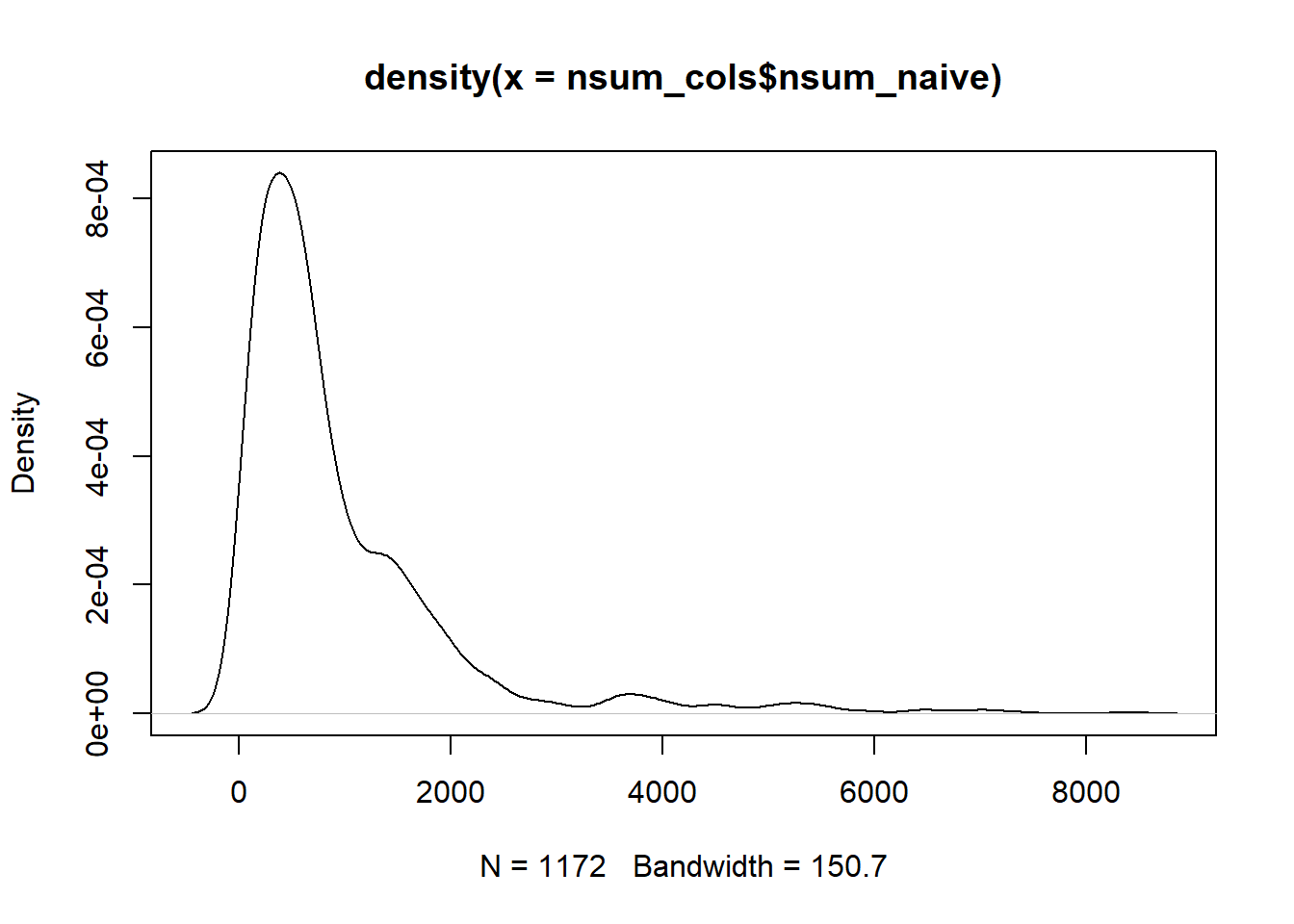

summary(nsum_cols$nsum_naive)

Compare this one with the one with downweighted minority group. e tweede density plot ziet er een stuk smoother uit. Dat lijkt positief. Nummers zijn wel een stuk hoger. Even controleren of dit enkel voor minderheden zou zijn of ook voor NL.

# network size of the 16 categories
for (i in 2:17) {
    nsum_cols_new[[paste0("size", i)]] <- (nsum_cols_new[[i]]/known_vector_new[i - 1]) * popsize  # naive numbers
}
# 2:20 21:39 average them
nsum_cols_new$nsum_naive <- rowMeans(nsum_cols_new[, c(18:33)])
nsum_cols_new <- nsum_cols_new[, -c(18:33)]
plot(density(nsum_cols_new$nsum_naive))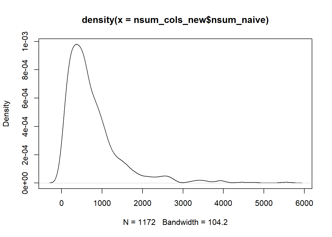

summary(nsum_cols_new$nsum_naive)

cor(nsum_cols_new$nsum_naive, nsum_cols$nsum_naive)

3.5 NSUM difficult

So how do we want to calculate? Through which column selections?

# new or not?  Let's start with the downweighing mat <- as.matrix(nsum_cols_new[,c(2:17)])
# known_vec <- known_vector_new colchoice <- 'downweighted/'


mat <- as.matrix(nsum_cols[, c(2:17)])
known_vec <- known_vector
colchoice <- "ibrahim/"

Now the hyperparameters in the Bayesian scenarios

iters <- 1000  # number of iterations (4k)
burns <- 500  # burnin size  (1k)
retain <- 500  # how many chains do we want to retain? (1k)
popsize <- 17407585  # population size
holdouts <- 1:length(known_vec)

Some parallel processing.

# paralellize the estimation
numCores <- detectCores()
if (numCores > length(holdouts - 1)) {
    registerDoParallel(cores = length(holdouts))
} else {
    print("Too few cores to do in one run!")
}

# register
registerDoParallel(core = numCores - 1)

Then the model itself, we run the combined model 16 times, each time holding out one known population, rendering it as “unknown”. We save 16 models, each time holding out one of the known populations as an “unknown” one.

# fill up empty lists
kds <- list()
kdssd <- list()
data_list <- list()

tic()
foreach(i = holdouts[15:16]) %dopar% { # change the number here on own max core you want to use #i = 1
  # 16 models to estimate. I use 7 cores, each core solves one per night.
  # so 16/7 = 2.3 = 3 nights.

  cd <- mat[, -c(i)] # take out pop of interest and make a new mat

  # calculate starting values
  z <- NSUM::killworth.start(
    cbind(cd, mat[, c(i)]), # paste the "takenout" at the END of matrix
    known_vec[-c(i)], # this is the known pop, WITHOUT unknown pop
    popsize
  ) # population size

  file_name_data <- paste0("Data/nsum_outcomes/", colchoice, "estimates_holdout", i, ".txt") # create file.name for data

  file_name_model <- paste0("Data/nsum_outcomes/", colchoice, "estimates_holdout", i, ".rds") # create file.name for model

  if (!file.exists(file_name_model)) { # check for file, if it does not exist run the NSUM model

    # run the Bayesian estimation
    degree <- NSUM::nsum.mcmc(cbind(cd, mat[, c(i)]), # gets pasted at the last column
      known_vector[-c(i)], # here we again take out the "holdout", or artificial "unknown" pop
      popsize,
      model = "combined", # combined control for transmission and recall errors
      indices.k = length(holdouts), # notice that "holdout" gets pasted as last column
      iterations = iters, burnin = burns, size = retain, # 40k iterations, retain 4k chains
      d.start = z$d.start, mu.start = z$mu.start, # starting values from simple estimator
      sigma.start = z$sigma.start, NK.start = z$NK.start
    )

    # store model_results
    save(degree, file = file_name_model)
  } else {
    load(file_name_model)
  }

  # store mean and sd in df
  # calculate rowmean and it's SD of the retained 4k chains
  kds[[i]] <- rowMeans(degree$d.values, na.rm = TRUE) # calculate rowmean of netsize iterations: so the retained chains
  kdssd[[i]] <- matrixStats::rowSds(degree$d.values) # calculate sd of 4k estimates per row: sd for those values
  data_list[[i]] <- data.frame(cbind(kds[[i]], kdssd[[i]])) # combine and put in df

  # Save the data, new .txt for each iteration, if something goes wrong, we can always start at prior one and combine
  write.table(data_list[[i]], file = file_name_data, row.names = F) # store them in results.
}
toc()
# 72 seconds for 100 iters
# 900 seconds for 1000 iters? --> quite linear

We next want to read the scenarios and compare them. What are their correlations?

# get all filenames of nsum bayes outcomes we want to do this for both secnarios: Ibrahim, and
# averages ethnic categories
filenames <- list.files(paste0("Data/nsum_outcomes/", colchoice), pattern = "*.txt", full.names = TRUE)

# read them into a list
ldf <- lapply(filenames, read.csv, header = T, sep = " ")

# remove calculated SD over the retained chains (OPTIONAL)
for (i in 1:length(ldf)) {
    ldf[[i]] <- data.frame(ldf[[i]][, c(1)])
}

# bind by column
df <- bind_cols(ldf, .name_repair = c("minimal"))

# names
names(df) <- c("scen1", "scen2", "scen3", "scen4", "scen5", "scen6", "scen7", "scen8", "scen9", "scen10",
    "scen11", "scen12", "scen13", "scen14", "scen15", "scen16")

# rowmeans
df$nsum_bayes <- rowMeans(df)
plot(density(df$nsum_bayes))
summary(df$nsum_bayes)

save(df, file = "Data/nsum_outcomes/df_ib.rda")


# df <- df[!df$nsum_bayes > describe(df$nsum_bayes)[[3]]+(3*describe(df$nsum_bayes)[[4]]),] #
# similar to TJ

# only for downweighted df_dw <- df save(df_dw, file = 'Data/nsum_outcomes/df_dw.rda')

Next, we want to calculate diversity and homogeneity metrics.

# sum of all answers
nsum_vars$sum_answers <- rowSums(nsum_vars[, c(2:24)])

# simple count of number unique NSUM 'i know a person in x-category' anwers
nsum_vars$count_answers <- rowSums(nsum_vars[, c(2:24)] != 0)

# function to calculate HH index over a dataframe input is dataframe with only nsum answers
fhhi <- function(df) {

    hhil <- list()  # list to fill
    hhi <- NULL  # outcome to fill
    for (i in 1:nrow(df)) {
        # over the rows of df with nsum answers

        # we extract the row and transpose it to get a column with all nsum answers
        hhil[[i]] <- data.frame(t(df[i, ]))

        # we then calculate the share of an nsum x (answers/total persons known) and we square that
        # to get the squared shares
        hhil[[i]][["ss"]] <- (hhil[[i]][, c(1)]/colSums(hhil[[i]]))^2

        # we then sum that column, to get the sum of squared shares, or the HHI
        hhi[i] <- sum(hhil[[i]][["ss"]])

    }
    return(hhi)  # return that info
}

# HHI over all answers
nsum_vars$hhi_answers <- fhhi(nsum_vars[, c(2:24)])

# HHI over dutch / moroc / turk
nsum_vars$nsum_dut <- rowSums(nsum_vars[, 2:9])
nsum_vars$nsum_mor <- nsum_vars$knows_mohammed + nsum_vars$knows_fatima
nsum_vars$nsum_tur <- nsum_vars$knows_ibrahim + nsum_vars$knows_esra

nsum_vars$hhi_ethnic <- fhhi(nsum_vars[, c("nsum_dut", "nsum_mor", "nsum_tur")])

# HHI over majority / minority
nsum_vars$nsum_min <- nsum_vars$nsum_mor + nsum_vars$nsum_tur
nsum_vars$hhi_majmin <- fhhi(nsum_vars[, c("nsum_dut", "nsum_min")])

# HHI over gender
nsum_vars$nsum_men <- nsum_vars$knows_daan + nsum_vars$knows_kevin + nsum_vars$knows_edwin + nsum_vars$knows_albert +
    nsum_vars$knows_mohammed + nsum_vars$knows_ibrahim
nsum_vars$nsum_women <- nsum_vars$knows_emma + nsum_vars$knows_linda + nsum_vars$knows_ingrid + nsum_vars$knows_willemina +
    nsum_vars$knows_fatima + nsum_vars$knows_esra
nsum_vars$hhi_gender <- fhhi(nsum_vars[, c("nsum_men", "nsum_women")])

# HHI over education
nsum_vars$hhi_educ <- fhhi(nsum_vars[, c("knows_university", "knows_hbo", "knows_mbo", "knows_secundary")])

# share women
nsum_vars$share_women <- nsum_vars$nsum_women/(nsum_vars$nsum_men + nsum_vars$nsum_women)

# share men
nsum_vars$share_men <- nsum_vars$nsum_men/(nsum_vars$nsum_men + nsum_vars$nsum_women)

# share dutch
nsum_vars$share_dut <- nsum_vars$nsum_dut/(nsum_vars$nsum_dut + nsum_vars$nsum_min)

# share minority
nsum_vars$share_min <- nsum_vars$nsum_min/(nsum_vars$nsum_dut + nsum_vars$nsum_min)

# share moroc
nsum_vars$share_mor <- nsum_vars$nsum_mor/(nsum_vars$nsum_dut + nsum_vars$nsum_min)

# share moroc
nsum_vars$share_tur <- nsum_vars$nsum_tur/(nsum_vars$nsum_dut + nsum_vars$nsum_min)

# share uni
nsum_vars$share_uni <- nsum_vars$knows_university/(nsum_vars$knows_university + nsum_vars$knows_hbo +
    nsum_vars$knows_mbo + nsum_vars$knows_secundary)

# share hbo
nsum_vars$share_hbo <- nsum_vars$knows_hbo/(nsum_vars$knows_university + nsum_vars$knows_hbo + nsum_vars$knows_mbo +
    nsum_vars$knows_secundary)

# share mbo
nsum_vars$share_mbo <- nsum_vars$knows_mbo/(nsum_vars$knows_university + nsum_vars$knows_hbo + nsum_vars$knows_mbo +
    nsum_vars$knows_secundary)

# share sec
nsum_vars$share_sec <- nsum_vars$knows_secundary/(nsum_vars$knows_university + nsum_vars$knows_hbo +
    nsum_vars$knows_mbo + nsum_vars$knows_secundary)

nsum_vars$nsum_uni <- nsum_vars$knows_university
nsum_vars$nsum_hbo <- nsum_vars$knows_hbo
nsum_vars$nsum_mbo <- nsum_vars$knows_mbo
nsum_vars$nsum_sec <- nsum_vars$knows_secundary

# diversity indices
new_df <- nsum_vars[, c("crespnr", "nsum_men", "nsum_women", "share_women", "share_men", "hhi_gender",
    "nsum_uni", "nsum_hbo", "nsum_mbo", "nsum_sec", "share_uni", "share_hbo", "share_mbo", "share_sec",
    "hhi_educ", "nsum_dut", "nsum_mor", "nsum_tur", "share_dut", "share_mor", "share_tur", "hhi_ethnic",
    "nsum_min", "share_min", "hhi_majmin")]

# match to NSUM with ibrahim as minority
nsum_cols$nsum_naive_ib <- nsum_cols$nsum_naive
# df$nsum_bayes_ib <- df$nsum_bayes

# only downweighted
nsum_cols_new$nsum_naive_dw <- nsum_cols_new$nsum_naive
# load('Data/nsum_outcomes/df_dw.rda') df_dw$nsum_bayes_dw <- df_dw$nsum_bayes

# new_df <- cbind(new_df, nsum_cols[,c('nsum_naive_ib')], df[,c('nsum_bayes_ib')],
# nsum_cols_new[,c('nsum_naive_dw')], df_dw[,c('nsum_bayes_dw')])
new_df <- cbind(new_df, nsum_cols[, c("nsum_naive_ib")], nsum_cols_new[, c("nsum_naive_dw")])
# names(new_df)[27] <-'nsum_bayes_ib' names(new_df)[29] <-'nsum_bayes_dw'
# cor(new_df[,c('nsum_naive_ib', 'nsum_naive_dw', 'nsum_bayes_ib', 'nsum_bayes_dw')]) save(new_df,
# file = 'Data/nsum_outcomes/nsum_size_diversity.rda')


# load(file = 'Data/nsum_outcomes/nsum_size_diversity.rda') rm(new_df)

dfans <- nsum_cols_new[, -c(1)]
means <- colMeans(dfans)

pops <- known_vector_new



fig <- data.frame(cbind(means, pops))
cor(fig)

cor(fig[!fig$pops > 750000, ])
cor(fig[!fig$pops > 250000, ])



ex1 <- ggplot(fig, aes(x = pops, y = means)) + geom_point() + xlim(x = c(0, 40000)) + geom_smooth(method = "lm") +
    geom_text(label = rownames(fig), nudge_y = 0.1) + theme_minimal() + xlab("Population size") + ylab("Average number mentioned") +
    sm_statCorr() + ggtitle("A) Population size <40k")
ex1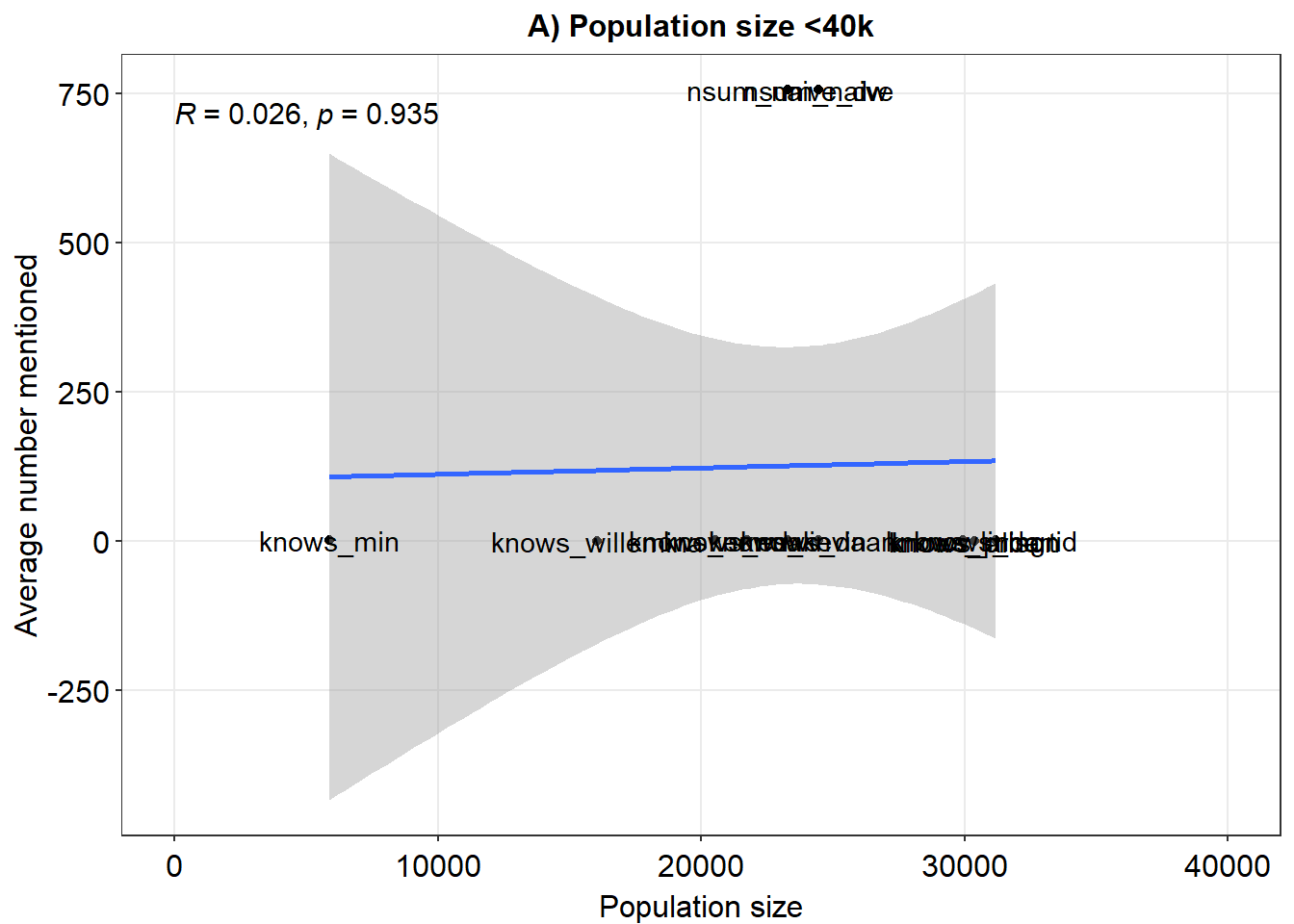

ex2 <- ggplot(fig, aes(x = pops, y = means)) + geom_point() + xlim(x = c(0, 550000)) + geom_smooth(method = "lm") +
    geom_text(label = rownames(fig), nudge_y = 0.1) + theme_minimal() + xlab("Population size") + ylab("Average number mentioned") +
    sm_statCorr() + ggtitle("B) Population size <550k")
ex2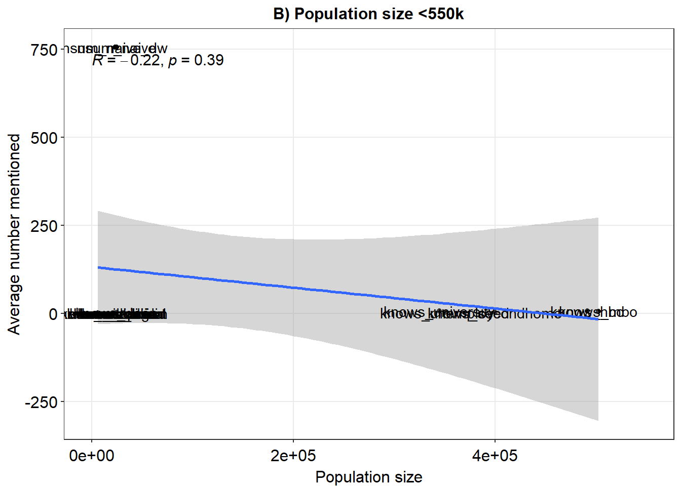

ex3 <- ggplot(fig, aes(x = pops, y = means)) + geom_point() + geom_smooth(method = "lm") + geom_text(label = rownames(fig),
    nudge_y = 0.1) + theme_minimal() + xlab("Population size") + ylab("Average number mentioned") + sm_statCorr() +
    ggtitle("C) All population sizes")
ex3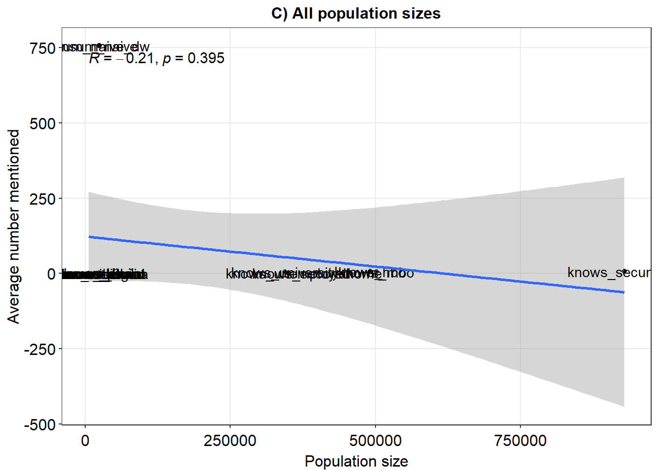

# ex <- plot_grid(ex1,ex2,ex3, nrow = 1) ex #ggsave('recall_populations.pdf', plot = ex, device =
# 'pdf', scale = 1, width = 16, height = 5, units = c('in'), dpi = 'retina')

#>            means       pops
#> means  1.0000000 -0.2133934
#> pops  -0.2133934  1.0000000
#>            means       pops
#> means  1.0000000 -0.2229974
#> pops  -0.2229974  1.0000000
#>           means      pops
#> means 1.0000000 0.0262563
#> pops  0.0262563 1.0000000

dfans <- nsum_cols_new[,-c(1)]
pops <- known_vector_new

# Analyze an example ard data set using Zheng et al. (2006) models
ard <- as.matrix(dfans)
subpop_sizes <- pops
known_ind <- c(1:16)
N <- 17407585

# indices
# 4 8 10 unpopular names
# 15  16 underrecalled
# 13 12 overrecalled

# first with primary scaling groups ALL
overdisp.est1 <- overdispersed(ard,
                            known_sizes = subpop_sizes[known_ind],
                            known_ind = known_ind,
                            G1_ind = known_ind,
                            N = N,
                            warmup = 1000,
                            iter = 10000)

# primary scaling groups all, except some
overdisp.est2 <- overdispersed(ard,
                            known_sizes = subpop_sizes[known_ind],
                            known_ind = known_ind,
                            G1_ind = c(4,8, 10), # underrecalled names
                            N = N,
                            warmup = 1000,
                            iter = 10000)

# primary scaling groups all, except some and others
overdisp.est3 <- overdispersed(ard,
                            known_sizes = subpop_sizes[known_ind],
                            known_ind = known_ind,
                            G1_ind = c(4,8, 10), # underrecalled names
                            G2_ind = c(15, 16), # underrecalled large cats
                            B2_ind = c(12, 13), # overrecalled large cats
                            N = N,
                            warmup = 1000,
                            iter = 10000)

# fewer than 20k
z <- which(subpop_sizes < 20000)
ard <- ard[, z]
subpop_sizes <- pops[z]
known_ind <- c(1:length(subpop_sizes))
overdisp.est4 <- overdispersed(ard,
                            known_sizes = subpop_sizes[known_ind],
                            known_ind = known_ind,
                            N = N,
                            warmup = 1000,
                            iter = 10000)


# only subpopulations < 50k (names, basically)
dfans <- nsum_cols_new[,-c(1)]
pops <- known_vector_new

ard <- as.matrix(dfans)
subpop_sizes <- pops
known_ind <- c(1:16)
N <- 17407585

z <- which(subpop_sizes < 50000)
ard <- ard[, z]
subpop_sizes <- pops[z]
known_ind <- c(1:length(subpop_sizes))
overdisp.est5 <- overdispersed(ard,
                            known_sizes = subpop_sizes[known_ind],
                            known_ind = known_ind,
                            G1_ind = known_ind,
                            N = N,
                            warmup = 1000,
                            iter = 10000)


# same iterations in one mean, correlate
x1 <- data.frame(colMeans(overdisp.est1$degrees))
x2 <- data.frame(colMeans(overdisp.est2$degrees))
x3 <- data.frame(colMeans(overdisp.est3$degrees))
x4 <- data.frame(colMeans(overdisp.est4$degrees))
x5 <- data.frame(colMeans(overdisp.est5$degrees))
summary(x1[,1])
summary(x2[,1])
summary(x3[,1])
summary(x4[,1])
summary(x5[,1])
x <- cbind(x1[,1],x2[,1], x3[,1], x4[,1], x5[,1])
cor(x)

#safe to data
new_df$netsover1 <- colMeans(overdisp.est1$degrees)
new_df$netsover2 <- colMeans(overdisp.est2$degrees)
new_df$netsover3 <- colMeans(overdisp.est3$degrees)
new_df$netsover4 <- colMeans(overdisp.est4$degrees)
new_df$netsover5 <- colMeans(overdisp.est5$degrees)

summary(new_df$netsover1)
summary(new_df$netsover2)
summary(new_df$netsover3)
summary(new_df$netsover4)
summary(new_df$netsover5)


#save(new_df, file = "Data/nsum_outcomes/nsum_size_diversity.rda")

nsum_df <- fload("Data/nsum_outcomes/nsum_size_diversity.rda")
cor(nsum_df[, c("netsover4", "netsover3", "nsum_naive_dw", "nsum_naive_ib")])

#>               netsover4 netsover3 nsum_naive_dw nsum_naive_ib
#> netsover4     1.0000000 0.5813190     0.8371885     0.8332478
#> netsover3     0.5813190 1.0000000     0.8885718     0.7314222
#> nsum_naive_dw 0.8371885 0.8885718     1.0000000     0.8916706
#> nsum_naive_ib 0.8332478 0.7314222     0.8916706     1.0000000

DiPrete, Thomas A., Andrew Gelman, Tyler McCormick, Julien Teitler, and Tian Zheng. 2011. “Segregation in Social Networks Based on Acquaintanceship and Trust.” American Journal of Sociology 116 (4): 1234–83. https://doi.org/10.1086/659100.

Jeroense, Thijmen, Bas Hofstra, Niels Spierings, and Jochem Tolsma. 2024. “Size and Ethnic Homogeneity of Extended Social Networks in the Netherlands: Differences Between Migrant Groups and Migrant Generations.” International Migration 63 (2). https://doi.org/10.1111/imig.13252.

---

Copyright © 2024- Bas Hofstra, Thijmen Jeroense, Jochem Tolsma